
 |
|||||
 |
|||||
Next: Estimation Procedure Up: Registration Algorithm Previous: Regularization Constraint
Transformation Parameterization
A 3D Fourier series representation[17] is used to parameterize
the forward and reverse transformations. This parameterization is simpler
than the parameterizations used in our previous work [14,28,29] and each basis coefficient can be
interpreted as the weight of a harmonic component in a single coordinate
direction. Let
![]() and
and
![]() . The displacement fields are defined to have the form
. The displacement fields are defined to have the form
![$\displaystyle u_c (x) = \sum_{k \in \Omega_d} \mu[k] e^{j<x,N \theta [k]>}$](img113.png) and
and![$\displaystyle \quad w_c (x) = \sum_{k \in \Omega_d} \eta[k] e^{j<x,N \theta [k]>}$](img114.png)
for
![$\displaystyle u_d [n] = u_c (\frac n N) = \sum_{k \in \Omega_d} \mu[k] e^{j<n,\theta [k]>}$](img121.png) and
and![$\displaystyle \quad w_d [n] = w_c (\frac n N) = \sum_{k \in \Omega_d} \eta[k] e^{j<n,\theta [k]>}$](img122.png)
for
The Fourier series parameterization is periodic in ![]() and therefore has cyclic boundary conditions for
and therefore has cyclic boundary conditions for ![]() on the boundary of
on the boundary of ![]() . Further more, the following proposition shows that the displacement
fields are real assuming that the coefficients
. Further more, the following proposition shows that the displacement
fields are real assuming that the coefficients ![]() and
and ![]() have complex conjugate symmetry. It is shown in Section 2.6
that
have complex conjugate symmetry. It is shown in Section 2.6
that ![]() and
and ![]() have complex conjugate symmetry by construction.
have complex conjugate symmetry by construction.
![$\displaystyle u_d [n] = 2 \sum_{k_1=0}^{(N_1/2)-1} \sum_{k_2=0}^{N_2-1} \sum_{k...
...^{j<n,\theta[k]>}\} - b[k] Im\{e^{j<n,\theta[k]>}\} \Big), \quad n \in \Omega_d$](img132.png) |
(8) |
if the
The displacement field
![$\displaystyle u_d [n] = \sum_{k \in \Omega_d} (a[k]+jb[k]) e^{j<n,\theta[k]>}
...
...}^{N_3-1}
(a[k]+jb[k])
e^{j<n,\theta[k]>}
+ (a[k]-jb[k]) e^{-j<n,\theta[k]>}
$](img136.png)
The Fourier series parameterization in Eq. 6
is useful for simplifying the linear elasticity constraint given in Eq. 5.
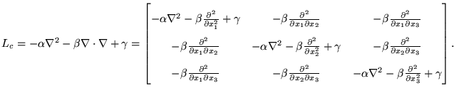
The operator ![]() can be thought of as a
can be thought of as a
![]() matrix differential operator[29] such that the linear elasticity operator
matrix differential operator[29] such that the linear elasticity operator
 Substituting Eq. 7
into Eq. 5 and discretizing2the continuous partial derivatives
of
Substituting Eq. 7
into Eq. 5 and discretizing2the continuous partial derivatives
of ![]() gives
gives
![$\displaystyle C_{\text{REG}}(u) + C_{\text{REG}}(w) = \sum_{k \in \Omega_d} \mu^{\dag }[k] D^2[k] \mu[k] + \eta^{\dag }[k] D^2[k] \eta[k]$](img146.png)
where
![$\displaystyle \Big[ D[k] \Big]_{rs} = \begin{cases}
2\alpha \Big\{ N_1^2 \big(1...
...big(\theta_r [k] \big)
\sin \big(\theta_s [k] \big) , & r \neq s .
\end{cases}$](img149.png)
Likewise, the inverse consistency constraint Eq. 3 can be simplified in a similar manner. Substituting Eq. 7 into Eq. 4 and discretizing gives
![$\displaystyle C_{\text{ICC}}(u,\tilde{w}) + C_{\text{ICC}}(w,\tilde{u}) = \sum_...
...ilde{\eta}[k]) +(\eta[k] - \tilde{\mu}[k])^{\dag } (\eta[k] - \tilde{\mu}[k]) .$](img150.png)
Next: Estimation Procedure Up: Registration Algorithm Previous: Regularization Constraint Xiujuan Geng 2002-07-04
Copyright © 2002 • The University of Iowa. All rights reserved.
Iowa City, Iowa 52242
Questions or Comments: gary-christensen@uiowa.edu