
 |
|||||
 |
|||||
Next: Regularization Constraint Up: Registration Algorithm Previous: Symmetric Similarity Cost Function
Inverse Consistency Constraint
Minimizing a symmetric cost function like Eq. 1
is not sufficient to guarantee that ![]() and
and ![]() are inverses of each other because the contributions of
are inverses of each other because the contributions of ![]() and
and ![]() to the cost function are independent. In order to couple the estimation
of
to the cost function are independent. In order to couple the estimation
of ![]() with that of
with that of ![]() , an inverse consistency constraint is imposed that is minimized when
, an inverse consistency constraint is imposed that is minimized when
![]() . The inverse consistency constraint is given by
. The inverse consistency constraint is given by
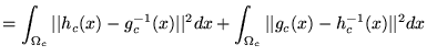
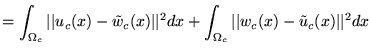
where
![$\displaystyle C_{\text{ICC}}(u , \tilde{w}) + C_{\text{ICC}}(w , \tilde{u}) = \...
...-\tilde{w}_d [n]\vert\vert^2 + \vert\vert w_d [n]-\tilde{u}_d [n]\vert\vert^2 .$](img81.png)
The procedure used to compute the inverse transformation of a transformation
with minimum Jacobian greater than zero is as follows. Assume that ![]() is a continuously differentiable transformation that maps
is a continuously differentiable transformation that maps ![]() onto
onto ![]() and has a positive Jacobian for all
and has a positive Jacobian for all
![]() . The fact that the Jacobian is positive at a point
. The fact that the Jacobian is positive at a point
![]() implies that it is locally one-to-one and therefore
has a local inverse. It is therefore possible to select a point
implies that it is locally one-to-one and therefore
has a local inverse. It is therefore possible to select a point
![]() and iteratively search for a point
and iteratively search for a point
![]() such that
such that
![]() is less than some threshold provided
that the initial guess of
is less than some threshold provided
that the initial guess of ![]() is close to the final value of
is close to the final value of ![]() .
.
The discretized inverse transformation is related to the continuous
inverse transformation by
![]() . This implies that the discrete inverse transformation
only needs to be calculated at each sample point
. This implies that the discrete inverse transformation
only needs to be calculated at each sample point
![]() . The following procedure is used to compute the discrete
inverse
. The following procedure is used to compute the discrete
inverse ![]() of the transformation
of the transformation ![]() .
.
For eachAs before,do {
Set,
, iteration = 0.
While (
threshold) do {
![$ \delta = \frac n N - h_d [N x]$](img92.png)

iteration = iteration + 1
if (iteration
Report algorithm failed to converge and exit.
}
![$ h_d^{-1} [n] = x$](img94.png)
}
Next: Regularization Constraint Up: Registration Algorithm Previous: Symmetric Similarity Cost Function Xiujuan Geng 2002-07-04
Copyright © 2002 • The University of Iowa. All rights reserved.
Iowa City, Iowa 52242
Questions or Comments: gary-christensen@uiowa.edu