Phantom, CT, and MRI Image Data

The inverse consistency and transitivity error of the transformations produced using the unidirectional and consistent linear-elastic algorithms were evaluated using phantom, CT, and MRI image data (see Figs. 3, 4 and 5)².

Figure 3: 2D phantoms used to test the image registration algorithms.

Phantom A	Phantom B	Phantom C

$\scalebox{0.70}{\includegraphics{trans_paper01.figs/phantoms/shepp_logan_128Tns000}}$	$\scalebox{0.70}{\includegraphics{trans_paper01.figs/phantoms/shepp_logan_128_warp1Tns000}}$	$\scalebox{0.70}{\includegraphics{trans_paper01.figs/phantoms/shepp_logan_128_warp2Tns000}}$

Figure 4: Axial slice 116 and sagittal slice 128 from the $256 \times 256 \times 200$ voxel CT data volume used to test the invertibility and transitivity of the image registration algorithms.

CT A	CT B	CT C
$\scalebox{0.375}{\includegraphics{trans_paper01.figs/skulls/FreeVa1_newtrSag128}}$	$\scalebox{0.375}{\includegraphics{trans_paper01.figs/skulls/WesselCa1_newtrSag128}}$	$\scalebox{0.375}{\includegraphics{trans_paper01.figs/skulls/WilliamsMa1_trSag128}}$
$\scalebox{0.375}{\includegraphics{trans_paper01.figs/skulls/FreeVa1_newtrTns116}}$	$\scalebox{0.375}{\includegraphics{trans_paper01.figs/skulls/WesselCa1_newtrTns116}}$	$\scalebox{0.375}{\includegraphics{trans_paper01.figs/skulls/WilliamsMa1_trTns116}}$

Figure 5: Original $256\times 320\times 256$ voxel MRI data volumes used to test the inverse consistency the image registration algorithms. Sagittal slice 128, and axial slice 145 are shown from top to bottom.

MRI A	MRI B	MRI C
$\scalebox{0.80}{\includegraphics{trans_paper01.figs/brains/b009_b104_b106_3x2small}}$

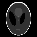
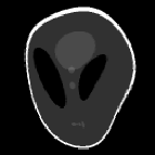
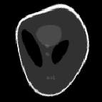
The phantom images were used to test how well the algorithms perform using simple shapes and how well they perform when images contain large regions of constant intensity. The dimensions of the phantoms were $128 \times 128$ pixel images. Phantoms B and C were generated from image A by deforming A with a random transformation such that the center of mass of the images remained in the center of the image.

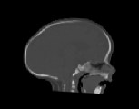
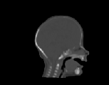
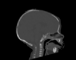
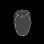
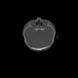
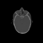
The CT images was used to test how well the algorithms perform when registering CT data of the head. Specifically, we were interested in how well the skull of one data set aligns with the skull of another data set for pre-operative surgical planning and post-operative evaluation. The CT images were collected from infants 3 months old and were selected such that there was a large shape difference between the heads. The CT image volumes A, B, and C were collected from a normal infant, an infant with bicoronal synostosis, and an infant with sagittal synostosis, respectively. The shape of the head in data set B is compressed front-to-back and the shape of the head in data set C is compressed side-to-side and elongated front-to-back. The CT data was resized and padded to make a $256 \times 256 \times 200$ voxels with voxel dimensions of 1 mm

. Each CT image volume was translated to align the sella turcica to voxel location

and rotated to align the Frankfort Horizontal plane of the skull to the voxel lattice using the procedure described in [33]. The intensity range of the data was reduced from 16-bits to 8-bits using a linear window that mapped the CT units of 600-2200 to the range 0-255.

The MRI brain data was used to test how well the algorithms perform on image volumes with complex-shape global and local anatomical structure. Each MRI was manually edited to remove soft tissue, skull, and the spinal cord. The MRI data sets were translated to align the anterior commissure (AC) point with voxel location

and rotated to align the midsagittal plane and the transverse plane containing the anterior and posterior commissures with the voxel lattice. The MRI data was resized and padded to create a $256 \times 256 \times 320$ voxel volume with voxel dimension 1 mm

. The intensity of the MRI data was converted from 16-bits to 8-bits such that all of the MRI data sets had roughly the same shaped intensity histograms.