Results

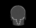
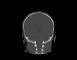
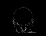
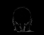
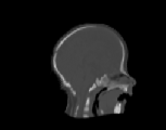
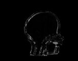
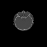
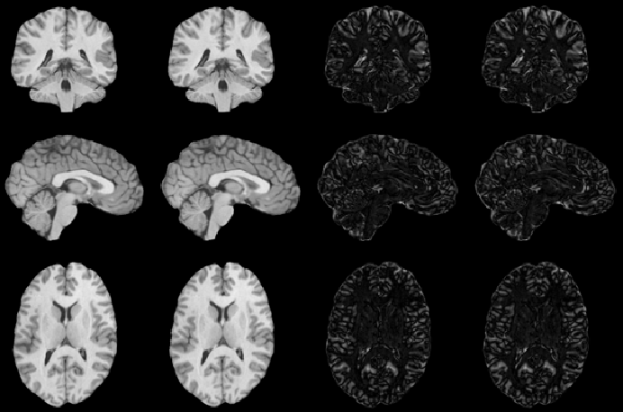
The inverse consistency and transitivity analysis was performed on three 2D phantom, three 3D CT, and 23 3D MRI data sets. The forward and reverse transformations between each pair of images were estimated using the unidirectional and consistent linear-elastic registration algorithms for each image modality. The image registration protocol used to register the phantom, CT and MRI images is described in Appendix A. All data sets were rigidly registered before being elastically registered. Typical transformation results for the phantom, CT and MRI data sets are presented in Figs. 6, 7 and 8. The CT and MRI figures show coronal, midsagittal, and transverse image slices from the 3D A-to-B registrations for the CT and MRI image registration experiments. These images represent the typical performance of the unidirectional and consistent linear-elastic image registration algorithms. Both figures show that the unidirectional and consistent algorithms produce very similar results with respect to matching image intensity. The difference images show that most of the matching error occurs at the edges of the images. This registration error is partially due to the fact that the linear-elastic model can only accommodate global nonrigid shape differences. The misregistration at the edges is also due to the balancing of the similarity and the regularization terms in the minimization problems defined by Eqs. 5 and 7. This occurs in both the unidirectional and consistent linear-elastic algorithms because the regularization term prevents the template image from fully deforming into the target data.

Figure 6: Column (a) shows the deformed phantom images produced by the unidirectional and ICC linear-elastic registration algorithms, for the data sets shown in Fig. 3. Column (b) shows the absolute magnitude difference between the deformed phantom images and the target images. Column (c) shows the magnitude inverse consistency constraint (ICC) error and column (d) shows the magnitude transitivity error. The top row shows the results for the unidirectional algorithm and the bottom row shows the results for the inverse consistent algorithm. The color bars are in units of pixels.

	A-to-B Transformed Images	A-to-B Mag.Intensity Difference	A-B-A Mag. ICC Error	A-B-C-A Mag. Trans. Error
	(a)	(b)	(c)	(d)

Figure 7: Columns (a) and (b) show transformed CT images resulting from the 3D unidirectional and ICC linear-elastic transformation of CT data set A to B, respectively, for the data sets shown in Fig. 4. Columns (c) and (d) show absolute difference images between the images in columns (a) and (b) with their respective slice from the target data set B. The rows correspond to views in the coronal, sagittal, and transverse orientations through the 3D volumes.

$A$-to-$B$ Transformed MRI (unidirectional)	$A$-to-$B$ Transformed MRI (ICC)	$\vert\vert T_A(h_{AB}(x)) - T_B(x)\vert\vert$ Abs. Intensity Diff. (unidirectional)	$\vert\vert T_A(h_{AB}(x)) - T_B(x)\vert\vert$ Abs. Intensity Diff. (ICC)
(a)	(b)	(c)	(d)

Figure 8: Columns (a) and (b) show transformed MRI images resulting from the 3D unidirectional and ICC linear-elastic transformation of MRI data set A to B, respectively, for the data sets shown in Fig. 5. Columns (c) and (d) show absolute difference images between the images in columns (a) and (b) with their respective slice from the target data set B. The rows correspond to views in the coronal, sagittal, and transverse orientations through the 3D volumes.

$A$-to-$B$ Transformed MRI (unidirectional)	$A$-to-$B$ Transformed MRI (ICC)	$\vert\vert T_A(h_{AB}(x)) - T_B(x)\vert\vert$ Abs. Intensity Diff. (unidirectional)	$\vert\vert T_A(h_{AB}(x)) - T_B(x)\vert\vert$ Abs. Intensity Diff. (ICC)
(a)	(b)	(c)	(d)

Copyright © 2002 • The University of Iowa. All rights reserved. Iowa City, Iowa 52242
Questions or Comments: gary-christensen@uiowa.edu