
 |
|||||
 |
|||||
Next: Multiresolution Registration Up: Results Previous: Results
Parameter Evaluation
Two MRI and two CT image volumes were used to investigate the effect of varying the parameters used in the consistent image registration algorithm. The data sets were collected from different individuals using the same MR and CT machines and the same scan parameters. The MRI data sets correspond to two normal adults and the CT data sets correspond to two 3-month-old infants, one normal and one abnormal (bilateral coronal synostosis). The MRI and CT data sets were chosen to test registration algorithm when matching anatomies with similar and dissimilar shapes, respectively.
The MRI data were preprocessed by normalizing the image intensities,
correcting for translation and rotation, and segmenting the brain from
the head using Analyze![]() (Mayo Clinic, Rochester, MN). The translation aligned the anterior
commissure points, and the rotation aligned the corresponding axial and
sagittal planes containing the anterior and posterior commissure points,
respectively. The MRI data sets were down-sampled and zero padded to form
a
(Mayo Clinic, Rochester, MN). The translation aligned the anterior
commissure points, and the rotation aligned the corresponding axial and
sagittal planes containing the anterior and posterior commissure points,
respectively. The MRI data sets were down-sampled and zero padded to form
a
![]() voxel lattice. The CT data sets were corrected
for translation and rotation and down-sampled to form a
voxel lattice. The CT data sets were corrected
for translation and rotation and down-sampled to form a
![]() voxel lattice. The translation aligned the basion
skull landmarks, and the rotation aligned the corresponding Frankfort
Horizontal and midsagittal planes, respectively.
voxel lattice. The translation aligned the basion
skull landmarks, and the rotation aligned the corresponding Frankfort
Horizontal and midsagittal planes, respectively.
Tables 1 and 2
show the results of 32 experiments for to MRI-to-MRI and CT-to-CT registration,
respectively, as the weighting values ![]() and
and ![]() were varied. The weight for the similarity cost
were varied. The weight for the similarity cost ![]() was set to one for all of the experiments. The values of
was set to one for all of the experiments. The values of ![]() and
and ![]() ranged from 0.0 to 0.0125 and 0 to 5000 for the MRI-to-MRI experiments,
respectively. The values of
ranged from 0.0 to 0.0125 and 0 to 5000 for the MRI-to-MRI experiments,
respectively. The values of ![]() and
and ![]() ranged from 0.0 to 0.00125 and 0 to 1275 for the CT-to-CT experiments,
respectively. The gradient descent step size was set to 0.00004 for the
MRI experiments and 0.0001 for the CT experiments. The difference in the
parameters is due to the different intensity characteristics of each modality.
These ranges can be used as a guide for determining parameter settings
for registration of other modalities. We have found that there is no need
to adjust the parameters for additional data sets of the same modality.
ranged from 0.0 to 0.00125 and 0 to 1275 for the CT-to-CT experiments,
respectively. The gradient descent step size was set to 0.00004 for the
MRI experiments and 0.0001 for the CT experiments. The difference in the
parameters is due to the different intensity characteristics of each modality.
These ranges can be used as a guide for determining parameter settings
for registration of other modalities. We have found that there is no need
to adjust the parameters for additional data sets of the same modality.
The data sets were registered initially with zero and first order harmonics.
Each experiment was run for 1000 iterations unless the algorithm failed
to converge. After every 100th iteration, the maximum harmonic was increased
by one. Each experiment that ran for 1000 iterations took approximately
1.5 hours to run on an AlphaPC clone using a single 667 MHz, alpha 21264
processor. It is expected that this time can be significantly decreased
by optimizing the code and using a better optimization technique than
gradient descent. In some of the experiments the Jacobian of the transformation
went negative due to insufficient regularization or due to a bad choice
of parameters. In these cases, the experiments were stopped before the
Jacobian went negative to report the results. The numbers reported for
the Similarity cost
![]() , the linear elasticity cost
, the linear elasticity cost
![]() , and the inverse consistency cost
, and the inverse consistency cost
![]() , were scaled by 10,000 for presentation.
, were scaled by 10,000 for presentation.
Experiments MRI01 and CT01 correspond to unconstrained estimation in
which the forward and reverse transformations were estimated independently.
These experiments produced the worst registration results as evident by
the largest values of
![]() ,
,
![]() , and
, and
![]() in the respective tables. These experiments were stopped
before the
in the respective tables. These experiments were stopped
before the ![]() iteration because the Jacobian went negative during the gradient
descent. This was expected since the regularization terms help prevent
the Jacobian from going negative. The similarity cost is the lowest for
these experiments since the algorithm finds the best match between the
images without any constraint preventing the Jacobian from going negative.
iteration because the Jacobian went negative during the gradient
descent. This was expected since the regularization terms help prevent
the Jacobian from going negative. The similarity cost is the lowest for
these experiments since the algorithm finds the best match between the
images without any constraint preventing the Jacobian from going negative.
Experiments MRI05, MRI09, MRI13, CT05, CT09, and CT13 demonstrate the
effect of estimating the forward and reverse transformations independently
while varying ![]() the weight of the linear elastic cost. As before, the large difference
between the forward and reverse displacement fields as reported by
the weight of the linear elastic cost. As before, the large difference
between the forward and reverse displacement fields as reported by
![]() confirms that linear elasticity alone is not sufficient
to guarantee that the forward and reverse transformations are inverses
of one another. However, the linear elasticity constraint did improve
the transformation over the unconstrained case because the minimum Jacobian
and the inverse of the maximum Jacobian is far from being singular.
confirms that linear elasticity alone is not sufficient
to guarantee that the forward and reverse transformations are inverses
of one another. However, the linear elasticity constraint did improve
the transformation over the unconstrained case because the minimum Jacobian
and the inverse of the maximum Jacobian is far from being singular.
Experiments MRI02, MRI03, MRI04, CT02, CT03, and CT04 demonstrate the
effect of jointly estimating the forward and reverse transformations without
enforcing the linear elasticity constraint. The
![]() values for these experiments are much lower than the
previous cases since they are being minimized. The forward and reverse
transformations are inverses of each other when
values for these experiments are much lower than the
previous cases since they are being minimized. The forward and reverse
transformations are inverses of each other when
![]() are zero so that the smaller the costs
are zero so that the smaller the costs
![]() , the closer the transformations are to being inverses
of each other.
, the closer the transformations are to being inverses
of each other.
The remaining experiments show the effect of jointly estimating the forward and reverse transformations while varying the weights on both the linear elasticity constraint and the inverse consistency constraint. These experiments show that it is possible to find a set of parameters that produce better results using both constraints than only using one or none. Notice that increasing the constraint weights causes the similarity cost to increase indicating a worse intensity match between the images. At the same time, the worst case values of the Jacobian increase as the constraint weights increase indicating less spatial distortion. The optimal set of parameters should be chosen to provide a good intensity match while producing the least amount of spatial distortion as measured by the Jacobian and an acceptable level of inverse consistency error.
The time series statistics for experiments MRI11 and CT15 are shown
in Figures 3 and 4,
respectively. These graphs show that the gradient descent algorithm converged
for each set of transformation harmonics. In both cases, the similarity
cost
![]() decreased at each iteration while the prior terms increased
before decreasing. Notice that the inverse consistency constraint increased
as the images deformed for each particular harmonic resolution. Then when
the number of harmonics were increased, the inverse constraint decreased
before increasing again. This is due to the fact that a low-dimensional
Fourier series does not have the degrees of freedom to faithfully represent
the inverse of a low-dimensional Fourier series. This is seen by looking
at the high dimensionality of a Taylor series representation of the inverse
transformation. Finally, notice that the inverse consistency constraint
caused the extremal Jacobian values of the forward and reverse transformations
to track together. The extremal Jacobian values correspond to the worst
case distortions produced by the transformations.
decreased at each iteration while the prior terms increased
before decreasing. Notice that the inverse consistency constraint increased
as the images deformed for each particular harmonic resolution. Then when
the number of harmonics were increased, the inverse constraint decreased
before increasing again. This is due to the fact that a low-dimensional
Fourier series does not have the degrees of freedom to faithfully represent
the inverse of a low-dimensional Fourier series. This is seen by looking
at the high dimensionality of a Taylor series representation of the inverse
transformation. Finally, notice that the inverse consistency constraint
caused the extremal Jacobian values of the forward and reverse transformations
to track together. The extremal Jacobian values correspond to the worst
case distortions produced by the transformations.
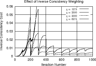
Figure 5
shows the effect of varying ![]() and
and ![]() on the inverse consistency cost
on the inverse consistency cost
![]() as a function of iteration. The left graph shows that
as a function of iteration. The left graph shows that
![]() increases with iteration and then drops every 100 iterations
when additional parameters (degrees of freedom) are added to the transformation.
The curves decrease in amplitude as
increases with iteration and then drops every 100 iterations
when additional parameters (degrees of freedom) are added to the transformation.
The curves decrease in amplitude as ![]() is increased until
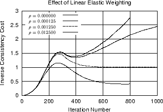
is increased until ![]() becomes to large and the algorithm fails to converge. The right
graph shows that
becomes to large and the algorithm fails to converge. The right
graph shows that
![]() increases as the linear elasticity weight
increases as the linear elasticity weight ![]() is increased. This makes sense because the two regularization
terms fight one another. The inverse consistency cost increases as the
linear elasticity cost is penalized more.
is increased. This makes sense because the two regularization
terms fight one another. The inverse consistency cost increases as the
linear elasticity cost is penalized more.
|
Next: Multiresolution Registration Up: Results Previous: Results Xiujuan Geng 2002-07-04
Copyright © 2002 • The University of Iowa. All rights reserved.
Iowa City, Iowa 52242
Questions or Comments: gary-christensen@uiowa.edu