55:148 Digital Image Processing
Chapter 4, Part III
Image Pre-processing: Local pre-processing
Related Reading
Sections from Chapter 4 according to the WWW Syllabus.
Chapter 4.3 Overview:
Local pre-processing
- Pre-processing methods use a small neighborhood of a pixel in an input image to get a
new brightness value in the output image.
- Such pre-processing operations are called also filtration.
- Local pre-processing methods can be divided into the two groups according to the goal of
the processing:
- Smoothing aims to suppress noise or other small fluctuations in the image
- equivalent to the suppression of high frequencies in the frequency domain.
- Unfortunately, smoothing also blurs all sharp edges that bear important information
about the image.
- Gradient operators are based on local derivatives of the image function.
- Derivatives are bigger at locations of the image where the image function undergoes
rapid changes. The aim of gradient operators is to indicate such locations in the image.
- Gradient operators have a similar effect as suppressing low frequencies in the frequency
domain.
- Noise is often high frequency in nature; unfortunately, if a gradient operator is
applied to an image the noise level increases simultaneously.
- Clearly, smoothing and gradient operators have conflicting aims.
- Some pre-processing algorithms solve this problem and permit smoothing and edge
enhancement simultaneously.
- Another classification of local pre-processing methods is according to the
transformation properties.
- Linear and nonlinear transformations can be distinguished.
- Linear operations calculate the resulting value in the output image pixel g(i,j) as a
linear combination of brightnesses in a local neighborhood of the pixel f(i,j) in the
input image.
- The contribution of the pixels in the neighborhood is weighted by coefficients h

- The above equation is equivalent to discrete convolution with the kernel h, that is
called a convolution mask.
- Rectangular neighborhoods O are often used with an odd number of pixels in rows and
columns, enabling the specification of the central pixel of the neighborhood.
- Local pre-processing methods typically use very little a priori knowledge about the
image contents. It is very difficult to infer this knowledge while an image is processed
as the known neighborhood O of the processed pixel is small.
- The choice of the local transformation, size, and shape of the neighborhood O depends
strongly on the size of objects in the processed image.
- If objects are rather large, an image can be enhanced by smoothing of small
degradations.
Image smoothing
- Image smoothing is the set of local pre-processing methods which have the aim of
suppressing image noise - it uses redundancy in the image data.
- Calculation of the new value is based on averaging of brightness values in some
neighborhood O.
- Smoothing poses the problem of blurring sharp edges in the image, and so we shall
concentrate on smoothing methods which are edge preserving. They are based on the
general idea that the average is computed only from those points in the neighborhood which
have similar properties to the processed point.
- Local image smoothing can effectively eliminate impulsive noise or degradations
appearing as thin stripes, but does not work if degradations are large blobs or thick
stripes.
Averaging
- Assume that the noise value
 at each pixel is
an independent random variable with zero mean and standard deviation
- We can obtain such an image by capturing the same static scene several times.
- The result of smoothing is an average of the same n points in these images g1,...,g{n}
with noise values
 {1},...,
 {n}
{n}

- The second term here describes the effect of the noise ... a random value with zero
mean.
- Thus if n images of the same scene are available, the smoothing can be accomplished
without blurring the image by

- In many cases only one image with noise is available, and averaging is then realized in
a local neighborhood.
- Results are acceptable if the noise is smaller in size than the smallest objects of
interest in the image, but blurring of edges is a serious disadvantage.
- Averaging is a special case of discrete convolution. For a 3 x 3 neighborhood the
convolution mask h is

- Larger convolution masks for averaging are created analogously.
Practical Experiment 4.D - VIP Version
- From VIP, open median.vip and save it in your account under a new name.
- Replace the Median filter with a general convolution (Convol node), you may use 'Find
Node' option to find the routine)
- Using the editor in the node properties box, create a 3x3 convolution mask that will
perform smoothing.
- Note: for the Convol node to work correctly, you must first convert the input data
to float or greater precision. This is necessary to avoid 'byte clipping'
- The following format must be followed:
- E.g., for a 3x3 averaging, the mask looks as follows (note that the sum of all
coefficients must be equal to one):
0.11 0.11 0.11
0.11 0.11 0.11
0.11 0.11 0.11
- Apply the 3x3 averaging mask to the corrupted image.
- Create 7x7 and 11x11 averaging masks and use them for averaging.
- Assess their smoothing and edge blurring performance.
- Experiment with noise of different severity:
- download the noiseGenerator.nod
node to generate Gaussian noise
- using the noise generator, create additive noise in the original image
- to change the standard deviation of the noise, you will have to use the multiply
node - think about what this means
- Should the noiseGenerator.nod node not be available due to technical reasons, use
the following test images in your project:
- Examples of additive Gaussian noise:
- Examples of binary shot noise:
Practical Experiment 4.D - Khoros Version
- From cantata, open the median.wksp and save it in your account under a new
name.
- Replace the Median filter with a general convolution (iconvolve), you may use
Edit->Find to find the routine)
- Using the editor, create a 3x3 convolution mask that will perform smoothing.
- The following format must be followed ... the convolution mask is a text file.
- E.g., for a 3x3 averaging, the mask looks as follows (note that the sum of all
coefficients must be equal to one):
0.11 0.11 0.11
0.11 0.11 0.11
0.11 0.11 0.11
- Apply the 3x3 averaging mask to the corrupted image.
- Create 7x7 and 11x11 averaging masks and use them for averaging.
- Assess their smoothing and edge blurring performance.
- Experiment with noise of different severity, experiment with other types of noise
(e.g., Gaussian).
- The significance of the central pixel may be increased to better reflect properties of
Gaussian noise.

Averaging with limited data validity
- Methods that average with limited data validity try to avoid blurring by averaging only
those pixels which satisfy some criterion, the aim being to prevent involving pixels that
are part of a separate feature.
- A very simple criterion is to use only pixels in the original image with brightness in a
predefined interval of invalid data [min,max].
- Consider a point (m,n) in the image. If the intensity at (m,n) has a valid intensity,
then nothing is done.
- However, if a point (m,n) has an invalid gray-level, then the convolution mask
is calculated in the neighborhood O from the nonlinear formula

Note that in the equation above, the interval min-max represents invalid data so that only
valid data is used in the averaging. Note that h(i,j) must be normalized by the number
of data values used in the mask.
- A second method performs the averaging only if the computed brightness change of a pixel
is in some predefined interval.
- This method permits repair to large-area errors resulting from slowly changing
brightness of the background without affecting the rest of the image.
- A third method uses edge strength (i.e., magnitude of a gradient) as a criterion.
- The magnitude of some gradient operator is first computed for the entire image, and only
pixels in the input image with a gradient magnitude smaller than a predefined threshold
are used in averaging.
Averaging according to inverse gradient
- The convolution mask is calculated at each pixel according to the inverse gradient.
- Brightness change within a region is usually smaller than between neighboring regions.
- Let (i,j) be the central pixel of a convolution mask with odd size; the inverse gradient
 at the point (m,n) with respect to (i,j) is
then

- If g(m,n) = g(i,j) then we define
 (i,j,m,n)
= 2;
- the inverse gradient
 is then in the
interval (0,2], and
  is smaller on the edge
than in the interior of a homogeneous region.
- Weight coefficients in the convolution mask h are normalized by the inverse gradient,
and the whole term is multiplied by 0.5 to keep brightness values in the original range.
- The constant 0.5 has the effect of assigning half the weight to the central pixel (i,j),
and the other half to its neighborhood.

- The convolution mask coefficient corresponding to the central pixel is defined as h(i,j)
= 0.5.
- The above method assumes sharp edges.
- When the convolution mask is close to an edge, pixels from the region have larger
coefficients than pixels near the edge, and it is not blurred. Isolated noise points
within homogeneous regions have small values of the inverse gradient; points from the
neighborhood take part in averaging and the noise is removed.
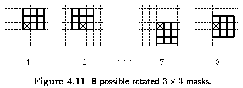
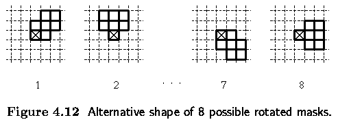
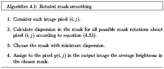
Averaging using a rotating mask
- avoids edge blurring by searching for the homogeneous part of the current pixel
neighborhood
- the resulting image is in fact sharpened
- brightness average is calculated only within the homogeneous region
- a brightness dispersion
 2 is
used as the region homogeneity measure.
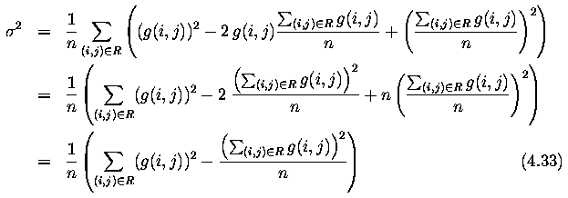
- let n be the number of pixels in a region R and g(i,j) be the input image. Dispersion
 2 is calculated as

- The computational complexity (number of multiplications) of the dispersion calculation
can be reduced if expressed as follows
Median smoothing
- In a set of ordered values, the median is the central value.
- Median filtering reduces blurring of edges.
- The idea is to replace the current point in the image by the median of the brightness in
its neighborhood.
- not affected by individual noise spikes
- eliminates impulsive noise quite well
- does not blur edges much and can be applied iteratively.
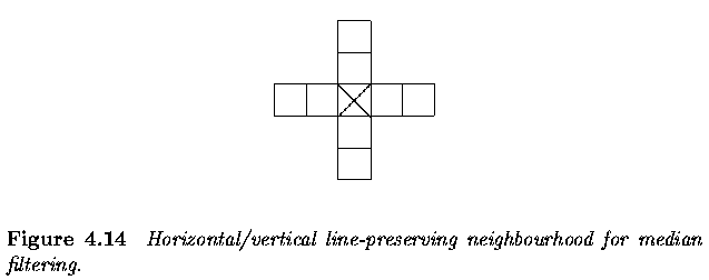
- The main disadvantage of median filtering in a rectangular neighborhood is its damaging
of thin lines and sharp corners in the image -- this can be avoided if another shape of
neighborhood is used.
Practical Experiment 4.E - VIP Version
- Remember median.vip?
- The original image Birds.gif that was corrupted with black and white lines can be
found here.
- You have 3 minutes to remove the lines from the image using median filtering - you
may need to experiment with the size of the median filter and/or with the number of
iterations.
- The goal is to remove the lines completely.
- Compare the median filter behavior if you use larger filter with less repetitions and
smaller filter with more repetitions.
- More examples to work with:
- Examples of additive Gaussian noise:
- Examples of binary shot noise:
Practical Experiment 4.E - Khoros Version
- Remember the median.wksp?
- The original image Birds.pgm that was corrupted with black and white lines can be
found in the images directory.
- You have 3 minutes to remove the lines from the image using median filtering - you
may need to experiment with the size of the median filter and/or with the number of
iterations.
- The goal is to remove the lines completely.
- Compare the median filter behavior if you use larger filter with less repetitions and
smaller filter with more repetitions.
Edge detectors
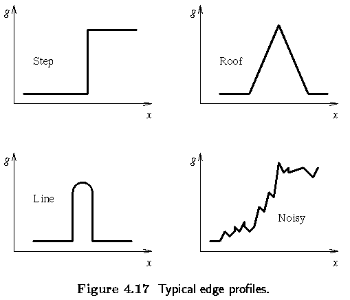
- locate sharp changes in the intensity function
- edges are pixels where brightness changes abruptly.
- Calculus describes changes of continuous functions using derivatives; an image function
depends on two variables - partial derivatives.
- A change of the image function can be described by a gradient that points in the
direction of the largest growth of the image function.
- An edge is a property attached to an individual pixel and is calculated from the image
function behavior in a neighborhood of the pixel.
- It is a vector variable
- magnitude of the gradient
- direction

- The gradient direction gives the direction of maximal growth of the function, e.g., from
black (f(i,j)=0) to white (f(i,j)=255).
- This is illustrated below; closed lines are lines of the same brightness.
- The orientation 0� points East.
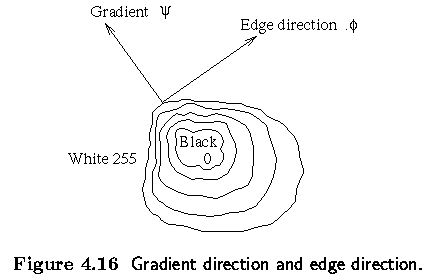
- Edges are often used in image analysis for finding region boundaries.
- Boundary and its parts (edges) are perpendicular to the direction of the gradient.
- The gradient magnitude and gradient direction are continuous image functions where
arg(x,y) is the angle (in radians) from the x-axis to the point (x,y).

- Sometimes we are interested only in edge magnitudes without regard to their
orientations.
- The Laplacian may be used.
- The Laplacian has the same properties in all directions and is therefore invariant to
rotation in the image.

- Image sharpening makes edges steeper -- the sharpened image is intended to be observed
by a human.
- C is a positive coefficient which gives the strength of sharpening and S(i,j) is a
measure of the image function sheerness that is calculated using a gradient operator.
- The Laplacian is very often used to estimate S(i,j).

Laplace operator
- The Laplace operator (Eq. 4.37) is a very popular operator approximating the second
derivative which gives the gradient magnitude only.
- The Laplacian is approximated in digital images by a convolution sum.
- A 3 x 3 mask for 4-neighborhoods and 8-neighborhood

- A Laplacian operator with stressed significance of the central pixel or its neighborhood
is sometimes used. In this approximation it loses invariance to rotation

- The Laplacian operator has a disadvantage -- it responds doubly to some edges in the
image.
Practical Experiment 4.F - VIP Version
- Using the above equation, create the convolution mask approximating the Laplacian.
- Use the Convol node to create the Laplacian edge image (see Pract.
exp. 4.D for convolution details).
- Use the Laplacian edge image for image sharpening as specified by (Eq. 4.38).
- Experiment with the value of the parameter C.
Practical Experiment 4.F - Khoros Version
- Using the above equation, create the convolution mask approximating the Laplacian.
- Use iconvolve to create Laplacian edge image (see Pract. exp. 4.D for
convolution details).
- Use the Laplacian edge image for image sharpening as specified by (Eq. 4.38).
- !!! IMPORTANT!!! -
- Define the kernel hotspot ... 1,1 for the 3x3 kernel (parameters within the iconvolve
routine), otherwise the convolution image will be shifted and the sharpening effect will
not be correct
- Use float data type - your first glyph should convert data from byte to float to
avoid overflow/underflow problems that are otherwise associated with the
convolution/subtraction process.
- Experiment with the value of the parameter C.
- Image sharpening / edge detection can be interpreted in the frequency domain as well.
- The result of the Fourier transform is a combination of harmonic functions.
- The derivative of the harmonic function sin (nx) is n cos (nx); thus the higher the
frequency, the higher the magnitude of its derivative.
- This is another explanation of why gradient operators enhance edges.
- Unsharp masking is often used in printing industry applications - another image
sharpening approach.
- A signal proportional to an unsharp image (e.g., blurred by some smoothing operator) is
subtracted from the original image, again a parameter C may be used to control the weight
of the subtraction.
Practical Experiment 4.G - VIP Version
- Using the above description, heavily smooth the image - you may use the lpfhpf.vip (used in the Introduction
chapter) or the averaging convolution filter designed in Pract. exp. 4.D).
- Subtract the smoothed image from the original (as you did in the first homework).
- Experiment with the values of the smoothing parameter and the parameter C.
Practical Experiment 4.G - Khoros Version
- Using the above description, heavily smooth the image - you may use the lpfhpf.wksp
(used in the Introduction chapter) or the averaging convolution filter designed in Pract.
exp. 4.D).
- Subtract the smoothed image from the original.
- Use float data type for subtraction.
- That includes not only the original image but also conversion of the complex data
resulting from the inverse FFT to float.
- Experiment with the values of the smoothing parameter and the parameter C.
- A digital image is discrete in nature ... derivatives must be approximated by differences.
- The first differences of the image g in the vertical direction (for fixed i) and in the
horizontal direction (for fixed j)

- n is a small integer, usually 1.
- The value n should be chosen small enough to provide a good approximation to the
derivative, but large enough to neglect unimportant changes in the image function.
- Symmetric expressions for the difference are not usually used because they neglect the
impact of the pixel (i,j) itself.

- Gradient operators can be divided into three categories
- I. Operators approximating derivatives of the image function using differences.
- rotationally invariant (e.g., Laplacian) need one convolution mask only.
- approximating first derivatives use several masks ... the orientation is estimated on
the basis of the best matching of several simple patterns.
- II. Operators based on the zero crossings of the image function second derivative (e.g.,
Marr-Hildreth or Canny edge detector).
- III. Operators which attempt to match an image function to a parametric model of edges.
- This category will not be covered here; parametric models describe edges more precisely
than simple edge magnitude and direction and are much more computationally intensive.
- Individual gradient operators that examine small local neighborhoods are in fact
convolutions and can be expressed by convolution masks.
- Operators which are able to detect edge direction as well are represented by a
collection of masks, each corresponding to a certain direction.
Roberts operator

- so the magnitude of the edge is computed as

- The primary disadvantage of the Roberts operator is its high sensitivity to noise,
because very few pixels are used to approximate the gradient.
Prewitt operator
- The Prewitt operator, similarly to the Sobel, Kirsch, Robinson (as discussed later) and
some other operators, approximates the first derivative.
- Operators approximating first derivative of an image function are sometimes called
compass operators because of the ability to determine gradient direction.
- The gradient is estimated in eight (for a 3 x 3 convolution mask) possible directions,
and the convolution result of greatest magnitude indicates the gradient direction. Larger
masks are possible.

- The direction of the gradient is given by the mask giving maximal response. This is
valid for all following operators approximating the first derivative.
Sobel operator

- Used as a simple detector of horizontality and verticality of edges in which case only
masks h1 and h3 are used.
- If the h1 response is y and the h3 response x, we might then
derive edge strength (magnitude) as

and direction as arctan (y / x).
Robinson operator

Kirsch operator

Practical Experiment 4.H - VIP Version
- Create the convolution masks corresponding to the 3x3 Prewitt edge detector
- create two masks, one of them corresponding to the South edge direction
(angle phi = 270 deg - look at Fig. 4.16),
- the second mask corresponding to the North-East direction (phi = 45
deg).
- Use the Convol node to detect edges in the S and NE directions
(see Pract. exp. 4.D for convolution details).
- To do this, place the Convol nodes with the masks you defined in parallel,
add the two images to combine the S and NE edges into a single resulting edge
image.
- To make sure that your edge detection masks give the correct direction,
use circle.jpg to test your masks.
- Apply to image sf.jpg and analyze
the results.
- What is the width of the edge responses?
- Now, add a thresholding node (download here,
and use 'Open->UserDefine node' to open it from the saved location) and
display only the significant edges of the edge image.
Practical Experiment 4.H - Khoros Version
- Create the convolution masks corresponding to the 3x3 Prewitt edge detector
- create two masks, one of them corresponding to the South edge direction (angle phi =
270 deg - look at Fig. 4.16),
- the second mask corresponding to the North-East direction (phi = 45 deg).
- Use iconvolve to detect edges in the S and NE directions (see Pract. exp. 4.D
for convolution details).
- To make sure that your edge detection masks give the correct direction, generate the
circle image from within Khoros and test your masks.
- Apply to image sf.pgm and analyze the results.
- What is the width of the edge responses?
- Now, add a thresholding glyph and display only the significant edges of the edge
image.
Marr-Hildreth Edge Detection:
Zero crossings of the second derivative
- Edge detection techniques like the Kirsch, Sobel, Prewitt operators are based on
convolution in very small neighborhoods and work well for specific images only.
- The main disadvantage of these edge detectors is their dependence on the size of objects
and sensitivity to noise.
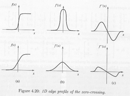
- The Marr-Hildreth edge detection technique, based on the zero crossings
of the second derivative explores the fact that a step edge corresponds to
an abrupt change in the image function.
- The first derivative of the image function should have an extreme at the position
corresponding to the edge in the image, and so the second derivative should be zero at the
same position.
- It is much easier and more precise to find a zero crossing position than
an extreme - see Fig. 4.20 in the book.
- Robust calculation of the 2nd derivative:
- smooth an image first (to reduce noise) and then compute second derivatives.
- The 2D Gaussian smoothing operator G(x,y)

- where x, y are the image co-ordinates and sigma is a standard deviation of the
associated probability distribution.
- The standard deviation sigma is the only parameter of the Gaussian filter - it is
proportional to the size of neighborhood on which the filter operates.
- Pixels more distant from the center of the operator have smaller influence, and pixels
further than 3 sigma from the center have negligible influence.
- Goal is to get second derivative of a smoothed 2D function f(x,y) ... the Laplacian
operator gives the second derivative, and is moreover non-directional (isotropic).
- Consider then the Laplacian of an image f(x,y) smoothed by a Gaussian ... LoG

- The order of differentiation and convolution can be interchanged due to linearity of the
operations:

- The derivative of the Gaussian filter is independent of the image under consideration
and can be precomputed analytically reducing the complexity of the composite operation.
- Using the substitution r2=x2+y2, where r measures
distance from the origin ( reasonable as the Gaussian is circularly symmetric, the 2D
Gaussian can be converted into a 1D function that is easier to differentiate.


- and the second derivative (LoG) is

- After returning to the original co-ordinates x, y and introducing a normalizing
multiplicative coefficient c (that includes 1/
 2),
we get a convolution mask of a zero crossing detector

where c normalizes the sum of mask elements to zero.
- Finding second derivatives in this way is very robust.
- Gaussian smoothing effectively suppresses the influence of the pixels that are up to a
distance 3 sigma from the current pixel; then the Laplace operator is an efficient and
stable measure of changes in the image.
- The location in the LoG image where the zero level is crossed corresponds to the
position of the edges.
- The advantage of this approach compared to classical edge operators of small size is
that a larger area surrounding the current pixel is taken into account; the influence of
more distant points decreases according to the
 of the Gaussian.
- The
 variation does not affect the location
of the zero crossings.
- Convolution masks become large for larger
 ;
for example,
  = 4 needs a mask about 40
pixels wide.
- The practical implication of Gaussian smoothing is that edges are found reliably.
- If only globally significant edges are required, the standard deviation
 of the Gaussian smoothing filter may be
increased, having the effect of suppressing less significant evidence.
- The LoG operator can be very effectively approximated by convolution with a mask that is
the difference of two Gaussian averaging masks with substantially different
 - this method is called the Difference of
Gaussians - DoG.
- Even coarser approximations to LoG are sometimes used - the image is filtered twice by
an averaging operator with smoothing masks of different size and the difference image is
produced.
- Disadvantages of zero-crossing:
- smoothes the shape too much; for example sharp corners are lost
- tends to create closed loops of edges
Practical Experiment 4.I - VIP Version
- The dog.vip project applies two Gaussian filters with 2 different values of
 .
.
- View the DoG image.
- Experiment with the smoothing parameters and with the thresholding parameters.
- The log.vip project computes the LoG image using the definition.
- Again try to experiment with the smoothing parameters and the thresholding
parameters.
- The one_step_log.vip project pre-computes the derivative of the Gaussian filter and
uses it (see p. 85 in the text).
- Apply the same projects to some other square image - e.g., lena.jpg - you may need to modify the smoothing
parameters.
Practical Experiment 4.I - Khoros Version
- Use the prepared workspace ZeroCross.wksp.
- This workspace applies two Gaussian filters with 2 different values of
 .
.
- View the DoG image.
- Experiment with the smoothing parameters and with the thresholding parameters
- Apply the same workspace to some other square image - e.g., Lena - you may need to
modify the smoothing parameters. Also, you may want to shrink the Lena image for faster
processing.
Scale in image processing
- Many image processing techniques work locally
- The essential problem in such computation is scale
- Edges correspond to the gradient of the image function that is computed as a difference
between pixels in some neighborhood
- There is seldom a sound reason for choosing a particular size of neighborhood
- The right size depends on the size of the objects under investigation.
- To know what the objects are assumes that it is clear how to interpret an image.
- This is not in general known at the pre-processing stage.
- Scale in image processing examples/solutions
- Processing of planar noisy curves at a range of scales - the segment of curve that
represents the underlying structure of the scene needs to be found.
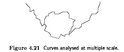
- After smoothing using the Gaussian filter with varying standard deviations, the
significant segments of the original curve can be found.
- The task can be formulated as an optimization problem in which two criteria are used
simultaneously
- the longer the curve segment the better
- the change of curvature should be minimal.
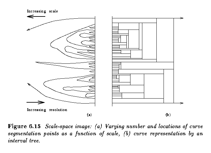
- Scale space filtering describes signals qualitatively with respect to scale.
- The original 1D signal f(x) is smoothed by convolution with a 1D Gaussian

- If the standard deviation
 is slowly
changed the following function represents a surface on the (x,
 ) plane that is called the scale--space image.
- Inflection points of the curve F(x,
 0)
for a distinct value
  0
0


- The positions of inflection points can be drawn as a set of curves in (x,
 ) co-ordinates.
- Coarse to fine analysis of the curves corresponding to inflection points, i.e., in the
direction of the decreasing value of the
 ,
localizes large-scale events.
- The qualitative information contained in the scale--space image can be transformed into
a simple interval tree that expresses the structure of the signal f(x) over all
observed scales.
- The interval tree is built from the root that corresponds to the largest scale.
- The scale-space image is searched in the direction of decreasing
 .
.
- The interval tree branches at those points where new curves corresponding to inflection
points appear.
- The third example of the application of scale - Canny edge detector.
Canny edge detection
- optimal for step edges corrupted by white noise
- optimality related to three criteria
- detection criterion ... important edges should not be missed, there should be no
spurious responses
- localization criterion ... distance between the actual and located position of the edge
should be minimal
- one response criterion ... minimizes multiple responses to a single edge (also partly
covered by the first criterion since when there are two responses to a single edge one of
them should be considered as false)
- Canny's edge detector is based on several ideas:
- 1) The edge detector was expressed for a 1D signal and the first
two optimality criteria. A closed form solution was found using the calculus of
variations.
- 2) If the third criterion (multiple responses) is added, the best
solution may be found by numerical optimization. The resulting filter can be approximated
effectively with error less than 20% by the first derivative of a Gaussian smoothing
filter with standard deviation
 ; the reason
for doing this is the existence of an effective implementation.
- There is a strong similarity here to the Marr-Hildreth edge detector (Laplacian of a
Gaussian)
- 3) The detector is then generalized to two dimensions. A step
edge is given by its position, orientation, and possibly magnitude (strength).
- It can be shown that convoluting an image with a symmetric 2D Gaussian and then
differentiating in the direction of the gradient (perpendicular to the edge direction)
forms a simple and effective directional operator.
- Recall that the Marr-Hildreth zero crossing operator does not give information about
edge direction as it uses Laplacian filter.
- Suppose G is a 2D Gaussian (equation 4.50) and assume we wish to convolute the image
with an operator Gn which is a first derivative of G in the direction n.

- The direction n should be oriented perpendicular to the edge
- this direction is not known in advance
- however, a robust estimate of it based on the smoothed gradient direction is available
- if g is the image, the normal to the edge is estimated as

- The edge location is then at the local maximum in the direction n of the operator
G_n convoluted with the image g

- Substituting in equation 4.62 for G_n from equation 4.60, we get

- This equation 4.63 shows how to find local maxima in the direction perpendicular to the
edge; this operation is often referred to as non-maximum suppression.
- As the convolution and derivative are associative operations in equation 4.63
- first convolute an image g with a symmetric Gaussian G
- then compute the directional second derivative using an estimate of the direction n
computed according to equation 4.61.
- strength of the edge (magnitude of the gradient of the image intensity function g) is
measured as

- 4) Spurious responses to the single edge caused by noise usually
create a so called 'streaking' problem that is very common in edge detection in
general.
- Output of an edge detector is usually thresholded to decide which edges are significant.
- Streaking means breaking up of the edge contour caused by the operator fluctuating above
and below the threshold.
- Streaking can be eliminated by thresholding with hysteresis.
- If any edge response is above a high threshold, those pixels constitute definite
output of the edge detector for a particular scale.
- Individual weak responses usually correspond to noise, but if these points are connected
to any of the pixels with strong responses they are more likely to be actual edges in the
image.
- Such connected pixels are treated as edge pixels if their response is above a low
threshold.
- The low and high thresholds are set according to an estimated signal to noise ratio.
- 5) The correct scale for the operator depends on the objects
contained in the image.
- The solution to this unknown is to use multiple scales and aggregate information from
them.
- Different scale for the Canny detector is represented by different standard deviations
 of the Gaussians.
- There may be several scales of operators that give significant responses to edges (i.e.,
signal to noise ratio above the threshold); in this case the operator with the smallest
scale is chosen as it gives the best localization of the edge.
- Feature synthesis approach.
- All significant edges from the operator with the smallest scale are marked first.
- Edges of a hypothetical operator with larger
 are synthesized from them (i.e., a prediction is made of how the large
  should perform on the evidence gleaned from the
smaller
  ).
).
- Then the synthesized edge response is compared with the actual edge response for larger
 .
.
- Additional edges are marked only if they have significantly stronger response than that
predicted from synthetic output.
- This procedure may be repeated for a sequence of scales, a cumulative edge map is built
by adding those edges that were not identified at smaller scales.
Algorithm: Canny edge detector
- Repeat steps (2) till (6) for ascending values of the standard deviation
 .
.
- Convolve an image g with a Gaussian of scale
 .
.
- Estimate local edge normal directions n using equation (4.61) for each pixel in
the image.
- Find the location of the edges using equation (4.63) (non-maximal suppression).
- Compute the magnitude of the edge using equation (4.64).
- Threshold edges in the image with hysteresis to eliminate spurious responses.
- Aggregate the final information about edges at multiple scale using the `feature
synthesis' approach.
- Canny's detector represents a complicated but major contribution to edge detection.
- Its full implementation is unusual, it being common to find implementations that omit
feature synthesis -- that is, just steps 2--6 of algorithm.
Practical Experiment 4.J - Windows Command-Line
Version
- Save the Canny.zip file from here.
- Extract the files to your home account.
- Open a command prompt window and traverse to the location where you extracted the
files.
- Type 'canny' at the prompt to see the usage instructions.
- Essentially, the syntax is as follows:
- canny image.gif sigma tlow thigh
- image: A GIF image upon which to perform Canny edge detection
- sigma: The standard deviation of the Gaussian kernel
- tlow: Fraction (0.0-1.0) of the high edge strength threshold
- thigh: Fraction(0.0-1.0) of the distribution of non-zero edge strengths for
hysteresis. The fraction is used to compute the high edge strength threshold
- the output edge image will be saved in the directory as image.gif_s_sigma_l_tlow_h_thigh.gif
- the bold items will be replaced by the values you chose earlier
- double-click on the output image of your choice to open it in Internet Explorer
- Experiment with these parameter settings on the following images:
- Try to get the most appropriate parameters for edge/border detection of finger bones
in the hand.gif image.
- You may wish also to compare the performance of the Canny edge detector on various
images with the performance of the Roberts and Sobel detectors that we saw in VIP earlier
in the semester.
Practical Experiment 4.J - Khoros Version
- From cantata, open the canny.wksp.
- You will see that the workspace provides comparison of the Canny edge detector (its
variation, to be exact) and the Sobel edge detector.
- Remember, there are 2 basic types of parameters in the Canny edge detector
- scale ... smoothing constant
 (in our
workspace, asymetric smoothing is allowed, there are 2 smoothing constants - set them to
equal values, use 5x5 or 7x7 mask size)
- thresholds for hysteresis thresholding
- In the provided implementation, an additional parameter can be set - the minimum
length of an edge response.
- Experiment with the parameter setting - experiment with the following images:
- clown.pgm
- hand.pgm
- uiowa.kdf ... you will have to convert this file to "byte" format first
- Try to get the most appropriate parameters for edge / border detection of finger
bones in the hand.pgm image
- What is the rationale for the 'edge response length' parameter?
Edges in multispectral images

Other local pre-processing operators
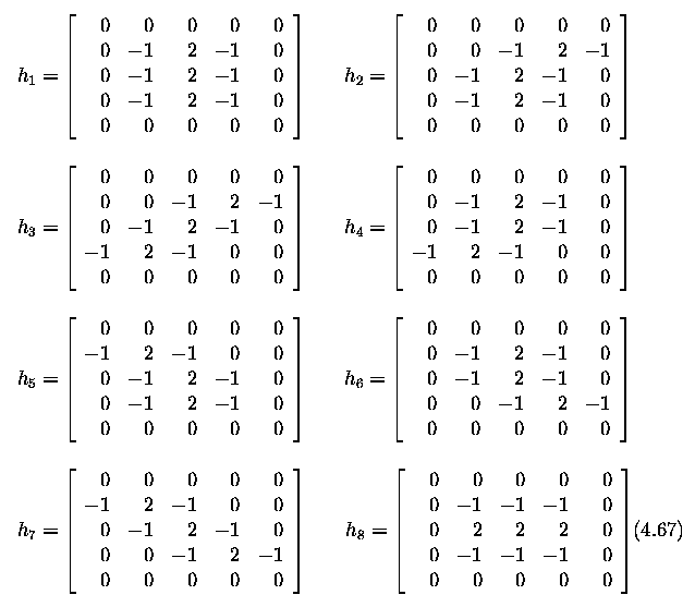
- Lines in the image can be detected by a number of local convolution operators - local
value is specified as:

- A set of 5 x 5 line detection masks:
Line Thining
- A binary image with edges that have magnitude higher than a threshold is
used as input.
- One denotes edge pixels and zeros the rest of the image.
- The following masks are used to thin the lines in the image. The letter
x denotes either a 0 or 1.
- The mask pattern is checked at each pixel in the image. If the mask matches,
the edge is thinned by replacing the pixel value in the center of the mask
by zero.

Edge Filling
- Edge points after thresholding do not create contiguous boundaries.
- Edge filling tries to recover edge pixels on the potential object boundary
which are missing.
- Local edge filling [Cervenka and Charvat 87] checks to see if the 3x3 neighborshood
of each pixel matches one of the patterns below.
- If there is a match, the central pixel of the neighborhood is changed from
a zero to a one.


Corner Dection with the Moravec Detector
- Input to the conrner dector is the gray-level image.
- Output is an image in which values are proportional to the likelihood that
the pixel is a corner.
- The Moravec detector is maximal in pixels with high contrast. These points
are on corners and sharp edges.

Parametric corner operator using the Zuniga-Haralick (ZH) operator
- The image function f is approximated in the neighborhood of the pixel (i,j)
by a cubic polynomial with coefficients c_k. This is a cubic facet model (Section
4.3.6).
- The ZH operator estimates the corner strength based on the coefficients
of the cubic facet model.
-


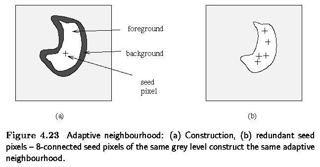
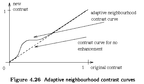
Adaptive neighboring pre-processing


[Back one section] [Table
of Contents] [Next Section]
Last Modified: August 31, 2000
![[Go Back]](../IMAGES/next.gif)


![]()


![]()


![]()


![]()



![]()
![]()


![]()


![]()

![]()


![]()

![]()

