55:148 Digital Image Processing

Homework

Check ICON for this semester's homework assignments. Homework assignments from 2008 appear below:

Assignment 10 (optional) - Hough-Transform

Due Wednesday, December 17, 2008 at or before 11:59 pm

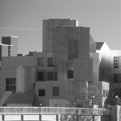
In this assignment you will use your image processing knowledge to implement an edge detection function that will be used in combination with a Hough-Transform for lines. The goal of the Hough-Transform step is to detect the 18 lines in Fig. 1 that subdivide the chessboard into 64 black/white fields.

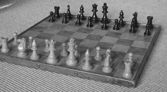
Fig. 1: Chessboard image (download).

You are to write an edge detection function called "hEdge(I)" that will be called by the program houghTrans.m (also download ht_plot2.m which is required by houghTrans.m). "I" represents the input image shown in Fig. 1. The function hEdge can consist of pre-processing, edge detection, and post-processing steps and must return a binary edge image which will be subsequently used for the Hough-Transform-based line detection step.

Optimize the function hEdge() so that the subsequent Hough-Transform step detects as many borderlines between the black and white chess fields as possible. Note that you are not allowed to make any changes to the files houghTrans.m or ht_plot2.m.

Submit your file hEdge.m and a short description of your design considerations.

Grading

You will be rewarded with n out of 18 possible points, where n represents the number of correctly segmented lines that represent dividing lines between the black and white chess fields in Fig. 1. For example, the result shown in Fig. 2 would yield 12 points; correctly detected lines are marked with green dots. Note that overlapping lines are counted only once.

Fig. 2

Deliverables
You will submit your completed assignment via the dropbox feature on the course ICON webpage. The files to be submitted include your completed .m file and a short paper describing your work. In your paper, discuss the design of your script and any problems you encountered. Discuss the results you obtained, specifically addressing the questions posed above. Finally, your paper should include a "conclusions" section, in which you describe what you learned from this assignment. Any common text format (MS Word, Open Office, .txt) is acceptable. NOTE: if you use Microsoft Office, please save the document in compatibility mode (*.doc, NOT *.docx) Collect all of your files in a single directory, compress the directory (.zip, .rar, .tar/gz), and submit it via ICON.

Assignment 9 - Image Restoration

Due Monday, December 08, 2008 at or before 11:59 pm

In this assignment you will use your image processing knowledge to repair a corrupted image:

Download this file. It is an RGB image; it consists of three monochrome channels, each representing one color in the image. Begin a matlab script with the following:

load('I.mat');

This will load the RGB image into a 512 x 512 x 3 matrix called 'I'. Suppose you wanted to access the red channel; this can be accomplished with I(:,:,1). Similarly, the blue channel can be found at I(:,:,3).

You are to write a program which constructs a restored RGB image. Note that you can use imshow(uint8(I), []) to display a double color image ' I '.

Deliverables
You will submit your completed assignment via the dropbox feature on the course ICON webpage. The files to be submitted include your completed .m file and a short paper describing your work. In your paper, discuss the design of your script and any problems you encountered. Discuss the results you obtained, specifically addressing the questions posed above. Finally, your paper should include a "conclusions" section, in which you describe what you learned from this assignment. Any common text format (MS Word, Open Office, .txt) is acceptable. NOTE: if you use Microsoft Office, please save the document in compatibility mode (*.doc, NOT *.docx) Collect all of your files in a single directory, compress the directory (.zip, .rar, .tar/gz), and submit it via ICON.

Assignment 7/8 - Laplacian of Gaussian

Due Monday, December 1, 2008 at or before 11:59 pm

In this assignment you will implement a second-derivative edge detector using the Laplacian of Gaussian (LoG) method described in Chapter 5 of the textbook. Your program will utilize a 2x2 zero-crossing detector to find edges in the LoG-processed image. In addition, to avoid detection of zero-crossings corresponding to non-significant edges, your program will use a first-derivative edge detector; this will provide supporting evidence of edges.

Test image - sc2.png:

Your solution is to be programmed in C++, using Matlab's MEX functionality. The following program shell is provided to help you get started: download. Extract this folder on your computer; it contains a skeleton Visual Studio solution, as well as two .m files: LoG.m contains parts of the MEX implementation, and test.m provides code to test your solution. All the files are in the proper locations; you only need to open "LoG.sln" in Visual Studio and complete the file "mexFunction.cpp".

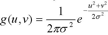
Your program should first compute the coefficients for a LoG kernel of arbitrary size using the following equation:

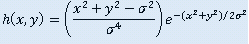
The value sigma will be passed to your program from Matlab. The following image may be helpful in computing your coefficients:

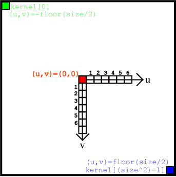
Assuming your kernel size is an odd number, the center value of the kernel corresponds to (u,v) = (0,0). Thus, in computing the coefficients, your (u,v) pairs should loop through the range: -floor(size/2) to floor(size/2). Check your coefficients to make sure they sum up to zero. If they do not sum to zero, you must fix them so they do; otherwise, your kernel will produce a response in homogeneous regions. Store the results of the computation in logKernel[].

After building your filter kernel, convolve your image with the LoG kernel, saving the result in logImage[]. Now, process this result image with a 2x2 zero-crossing detector. A zero crossing of a second derivative corresponds to a (possible) edge. The following image may be helpful:

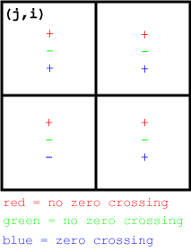
For every pixel in logImage[], analyse the 2x2 region defined such that the upper left pixel is the origin. If there is a sign change in the region, there is a zero-crossing. For all pixels that show proof of a zero-crossing, store a value of 'true' in the corresponding pixel of edges[].

Now, to provide additional robustness against spurious edge responses, process the original image with the following first-derivative edge detectors (in a manner similar to the horizontal and vertical Kirsch operators in the second part of HW5):

For every pixel, if the magnitude response (mag = sqrt(h1Response^2 + h2Response^2)) exceeds the threshold, *AND* the corresponding pixel of edges[] is 'true', then we have sufficient evidence of an edge. Write a value of 255 to the corresponding pixel of imageOut[] (all non-edge pixels should contain 0).

Your C++ program will be called from Matlab with 4 arguments: I, the image to be processed; SIZE, the size of the filter kernel; SIGMA, the standard deviation of the Gaussian function; THRESHOLD, a threshold to be used for determining valid edges.

To recap, you should do the following to implement your program:

1.) Write your BuildKernel() function. This will do the following:

Compute coefficients for the LoG kernel;
Verify that kernel coeffients sum up to zero;

2.) Convolve your input image with the LoG kernel:

Since you are accepting arbitrary kernel sizes, you need to pay close attention to your loop bounds;
Assign the results of this convolution to logImage[];

3.) Process logKernel[] with a 2x2 zero-crossing detector:

Loop through all pixels of logImage[];
If you see a sign change in the 2x2 region of interest, there is a zero-crossing (edges[] = true);

4.) Convolve your input image with the first-derivative kernels:

Convolve h1 and the input image;
Convolve h2 and the input image;
Assign magnitude[...] = sqrt(h1Response[...]^2 + h2Response[...]^2);
if (magnitude[...] > threshold && edges[...] == true), there is an edge;

Deliverables
You will submit your completed assignment via the dropbox feature on the course ICON webpage. The files to be submitted include your completed .m file and a short paper describing your work. In your paper, discuss the design of your script and any problems you encountered. Discuss the results you obtained, specifically addressing the questions posed above. Finally, your paper should include a "conclusions" section, in which you describe what you learned from this assignment. Any common text format (MS Word, Open Office, .txt) is acceptable. NOTE: if you use Microsoft Office, please save the document in compatibility mode (*.doc, NOT *.docx) Collect all of your files in a single directory, compress the directory (.zip, .rar, .tar/gz), and submit it via ICON.

Assignment 6 - Gaussian Smoothing Filter

Due Monday, November 10, 2008 at or before 11:59 pm

In this assignment you will implement a Gaussian smoothing filter in C++, using Matlab's MEX functionality. Start with the example presented in class on Oct. 23rd and 28th. You will modify the C++ code to implement a Gaussian filter with adjustable standard deviation (sigma) and filter size.

Your program should first compute the coefficients for a square Gaussian kernel (size x size) using the following equation:

The following image may be helpful in computing your kernel coefficients:

Assuming your kernel size is an odd number, the center value of the kernel corresponds to (u,v) = (0,0). Thus, in computing the coefficients, your (u,v) pairs should loop through the range: -floor(size/2) to floor(size/2).

Implement a Matlab mex-function of this form: GaussianFilter(imageIn, size, sigma). In addition, write a "test.m"-file in Matlab to test your implementation using the following image:

sc3.png:

Your mex-function in combination with the Matlab test function must implement a suitable boundary treatment approach of your choice; briefly discuss your approach.

Deliverables
You will submit your completed assignment via the dropbox feature on the course ICON webpage. The files to be submitted include your completed .m file and a short paper describing your work. In your paper, discuss the design of your script and any problems you encountered. Discuss the results you obtained, specifically addressing the questions posed above. Finally, your paper should include a "conclusions" section, in which you describe what you learned from this assignment. Any common text format (MS Word, Open Office, .txt) is acceptable. NOTE: if you use Microsoft Office, please save the document in compatibility mode (*.doc, NOT *.docx) Collect all of your files in a single directory, compress the directory (.zip, .rar, .tar/gz), and submit it via ICON.

Assignment 5 - Edge Detection

Due Monday, October 27, 2008 at or before 11:59 pm

In this assignment you will implement an edge detection algorithm using the Kirsch operator (textbook p. 138) in eight directions. First, define the Kirsch operator matrices, and compute the convolution of each of the operator matrices with the following image:

peppers.png:

The gradient direction is determined by the operator rotation giving the maximum response. Determine which operator rotation gives the greatest response. Store this magnitude in an image. Next, encode the corresponding gradient direction in another image using the following scheme:

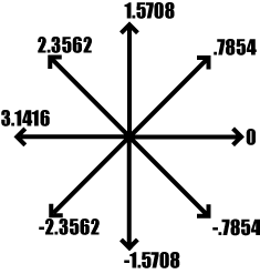
For regions in the image in which there is no edge, encode the gradient direction as '6'. Define a threshold such that all edge magnitude values below the threshold are encoded as "no edge".

Next, compute the gradient direction using only the response from the horizontal and vertical Kirsch operators (hint: atan2() may be helpful). Again, use a threshold to detect areas where no edge exists as above and store this information in an image. Compare the two schemes for calculating gradient direction. What are the differences?

Implement a suitable pre-processing step to reduce the impact of noise on the edge detection result and discuss your approach and results.

What is the relation between gradient direction and edge direction?

Deliverables
You will submit your completed assignment via the dropbox feature on the course ICON webpage. The files to be submitted include your completed .m file and a short paper describing your work. In your paper, discuss the design of your script and any problems you encountered. Discuss the results you obtained, specifically addressing the questions posed above. Finally, your paper should include a "conclusions" section, in which you describe what you learned from this assignment. Any common text format (MS Word, Open Office, .txt) is acceptable. NOTE: if you use Microsoft Office, please save the document in compatibility mode (*.doc, NOT *.docx) Collect all of your files in a single directory, compress the directory (.zip, .rar, .tar/gz), and submit it via ICON.

Assignment 4 - Geometric Transformations

Due Monday, October 20, 2008 at or before 11:59 pm

In this assignment, you will experiment with geometric image transformations. Imagine that you have been given images of the same scene, taken with different cameras. Suppose that the second camera delivers geometrically distorted images, and that the resulting images (A, B, and C) can't be directly overlaid on the image generated with the first camera ('lena-1.png'). In order to perform any sort of analysis of the images, you must first ensure that the images line up; this can be accomplished using geometric image transformations.

In this assignment, you are to write a Matlab script that will transform images A, B, and C to line up with the image 'lena-1.png'. Try to find the optimal geometric transformation for each of the images A, B, and C. Determine appropriate point mappings (corresponding points) between each pair of images. Note that impixelinfo( ) might be useful in this context; impixelinfo( ) can be called after imshow( ), allowing you to use the cursor to get pixel coordinates.

Construct and apply your transformation matrices using Matlab functions like maketform( ), cp2tform( ), or imtransform( ). A 'bilinear' gray-value interpolation method shall be used to generate the transformed image.

Crop your transformed images to match the size of the image 'lena-1.png'. Compare your result with the original image. How well does it line up? Try to analyze your transformation results and optimize the selection of the corresponding points.

Fig. 1: lena-1.png

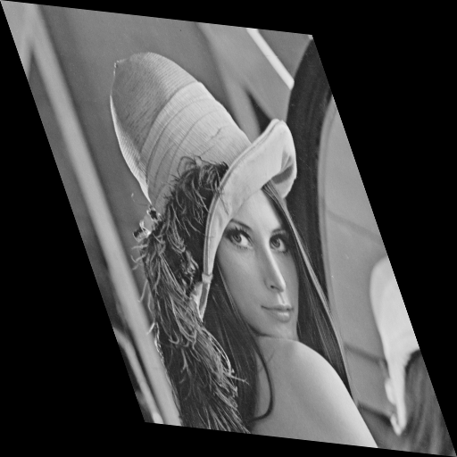Fig. 2: A.png

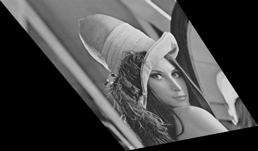Fig. 3: B.png

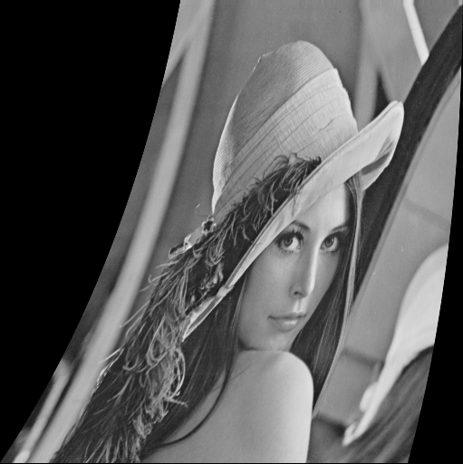Fig. 4: C.png

Deliverables
You will submit your completed assignment via the dropbox feature on the course ICON webpage. The files to be submitted include your completed .m file and a short paper describing your work. In your paper, discuss the design of your script and any problems you encountered. Discuss the results you obtained, specifically addressing the questions posed above. Finally, your paper should include a "conclusions" section, in which you describe what you learned from this assignment. Any common text format (MS Word, Open Office, .txt) is acceptable. Collect all of your files in a single directory, compress the directory (.zip, .rar, .tar/gz), and submit it via ICON.

Assignment 3 - Integral Images

Due Thursday, October 9, 2008 at or before 11:59 pm

Recall the integral image, a matrix representation that holds global image information. In this assignment, you will write a Matlab script to construct an integral image. The input image can be downloaded here (iitest.png). From this image you will construct the corresponding integral image using algorithm 4.2 from the textbook.

The advantage of the integral image is that it allows any rectangular sum to be computed with only four memory reads. This is useful in image feature calculation. In this assignment, you will evaluate a rectangular filter mask (Fig. 1) at different locations in the image (Fig. 2). Your mask is a hx8 rectangle, with positive and negative weighted pixel values according to Fig. 1.

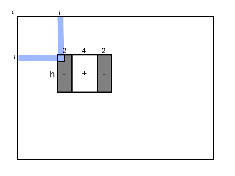
Fig. 1: Filter mask.

Write a Matlab function of this form: dipFeature(II, i, j, h); where II is the integral image, (i,j) is the pixel at which to evaluate the mask, and h defines the height of the mask. This function will compute and return the mean value of all positive and negative weighted pixel values of the mask (Fig. 1). The origin of the mask is defined to be the upper left corner.

Evaluate the filter mask response at the given coordinates (i,j) using the corresponding parameter h:

Position	i	j	h
1	60	47	8
2	148	60	8
3	20	99	8
4	30	149	8
5	50	180	8
6	170	139	16
7	170	20	1

Take care to evaluate the correct pixels in the integral image and minimize the number of integral image pixels accessed.

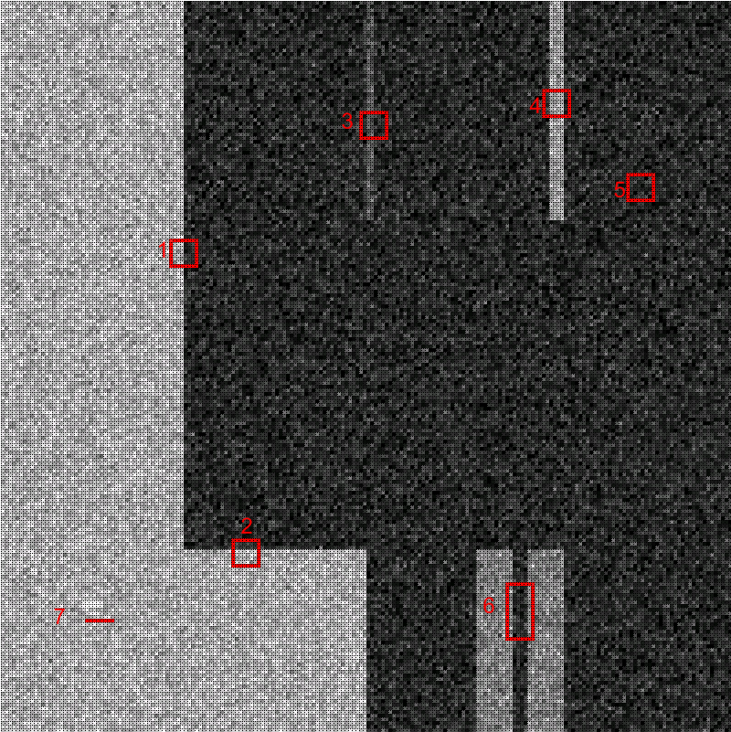
Fig. 2: Test image showing the location and size of the feature masks to evaluate.

What results do you obtain? Considering the pixel locations and the size of the mask, why did you get the results that you did? What can you say about the type of region that produces no response from the mask (i.e. it sums to approximately zero)? What can you say about the type of region that does produce a response from the mask? Does the computation time depend on the size of the mask?

Deliverables
You will submit your completed assignment via the dropbox feature on the course ICON webpage. The files to be submitted include your completed .m file and a short paper describing your work. In your paper, discuss the design of your script and any problems you encountered. Discuss the results you obtained, specifically addressing the questions posed above. Finally, your paper should include a "conclusions" section, in which you describe what you learned from this assignment. Any common text format (MS Word, Open Office, .txt) is acceptable. Collect all of your files in a single directory, compress the directory (.zip, .rar, .tar/gz), and submit it via ICON.

Assignment 2 - Color Images

Due Monday, September 29, 2008 at or before 11:59 pm

Electronic photosensitive sensors are monochromatic. To acquire color images, a color filter array (Bayer) mosaic is often combined with a single photosensitive sensor (e.g., CCD) to create a color camera. Figure 1 visualizes the raw sensor data of such a color camera. Color information is stored in the image according to the utilized Bayer filter mosaic (Fig. 2).

In this assignment, you are to write a Matlab m-file script to generate a color image (RGB color space) from the raw sensor data (sensor_data.png). Missing information in the three color channels must be generated by using an appropriate interpolation method. The upper left corner of the Bayer filter mosaic used in combination with the sensor is shown in Fig. 2.

Discuss the effect of the Bayer filter mosaic on image resolution. Outline your design considerations; specifically the choice of the interpolation method.

(a)

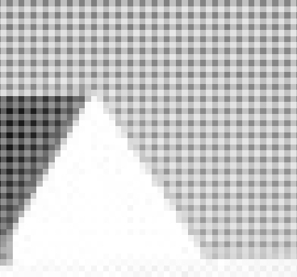(b)
Fig. 1: Raw sensor data of a color camera CCD sensor. (a) Full image and (b) magnified image part of (a).

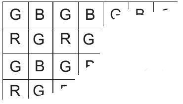
Fig. 2: Bayer filter mosaic.

Deliverables
You will submit your completed assignment via the dropbox feature on the course ICON webpage. The files to be submitted include your completed .m file and a short paper describing your work. In your paper, discuss the design of your script and any problems you encountered. Discuss the results you obtained, specifically addressing the questions posed above. Finally, your paper should include a "conclusions" section, in which you describe what you learned from this assignment. Any common text format (MS Word, Open Office, .txt) is acceptable. Collect all of your files in a single directory, compress the directory (.zip, .rar, .tar/gz), and submit it via ICON.

Assignment 1 - Image Reconstruction

Due Monday, September 15, 2008 at or before 11:59 pm

An interlaced camera transmits a full-resolution image by transmitting first the odd lines (rows) in the first frame (image) followed by the even lines of the image in the second consecutive frame. The full resolution image can be recovered by combining odd and even image frames accordingly (see Fig. 1).

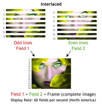
Fig. 1

In this assignment, you are to write a Matlab m-file script to assemble a full resolution image based on consecutive digitized odd and even image frames captured by an interlaced camera (Figs. 2 and 3).

Fig. 2: Odd image frame.

Fig. 3: Even image frame (disturbed see text).

In addition, it is known that the camera is faulty. The defect only effects the even image frames. In the transmission process, the pixel rows of the even frames appear shifted by the mean value of the row (subtraction of the row's mean from the original row pixel intensities). Your program must correct this disturbance so that the recovered full resolution image doesn't show any disturbances.

The two odd and even image frames are stored as Matlab 'mat' files and can be downloaded here: even corrupted frame; odd frame. To load the frames, use Matlab's "load" function (see 'help load'). A simple way to correct the image is to use the odd rows mean values and add them to the adjacent even row. Use Matlab's powerful array processing functions to perform the reconstruction. Avoid using loops! Once you are done with the function and have tested it, answer the following questions:

1. Why does this method work?

2. Can you suggest any other approaches that could be used to restore the origininal image?

Deliverables
You will submit your completed assignment via the drop-box feature on the course ICON webpage. The files to be submitted include your completed .m file and a short paper describing your work. In your paper, discuss the design of your script and any problems you encountered. Discuss the results you obtained, specifically addressing the questions posed above. Finally, your paper should include a "conclusions" section, in which you describe what you learned from this assignment. Any common text format (MS Word, Open Office, .txt) is acceptable. Collect all of your files in a single directory, compress the directory (.zip, .rar, .tar/gz), and submit it via ICON.

Last Modified: 2010