55:148 Digital Image Processing
55:247 Image Analysis and Understanding
Chapter 8, Part VII
Image understanding: Hidden Markov Models
Hidden Markov Models
- It is often possible when attempting image understanding to model the patterns
being observed as a transitionary system.
- Sometimes these are transitions in time, but they may also be transitions through
another pattern; for example, the patterns of individual characters when
connected in particular orders represent another pattern that is a word.
- If the transitions are well understood, and we know the system state at a certain
instant, they can be used to assist in determining the state at a subsequent point.
- One of the simplest examples is the Markov model.
- A Markov model assumes a system may occupy one of a finite number of states
X_1, X_2, X_3, ... , X_n at times t_1, t_2, ..., and that the
probability of occupying a state is determined solely by recent history.
- More specifically, a first-order Markov model assumes these probabilities
depend only on the preceding state; thus a matrix A will exist in which

- Thus 0 <= a_ij <= 1 and sum_j=1^n (a_ij) = 1 for all 1 <= i <= n.
- The important point is that these parameters are time independent -- the a_ij do
not vary with t.
- A second order model makes similar assumptions about probabilities depending on
the last two states, and the idea generalizes obviously to order k models
for k = 3,4, ...
- A trivial example might be to model weather forecasting: Suppose that the weather
on a given day may be sunny (1), cloudy (2) or rainy (3) and that
the day's weather depends probabilistically on the preceding day's weather only.
- We might be able to derive a matrix A

- so the probability of rain after a sunny day is 0.125, the probability of cloud
after a rainy day is 0.375 and so on.
- In many practical applications, the states are not directly observable, and instead
we observe a different set of states Y_1 , ... , Y_m (possibly n <= m) where
we can only guess the exact state of the system from the probabilities

- so 0<= b_jk <= 1 and sum_k=1^m (b_jk) = 1.
- The n x m matrix B is time independent; that is, the observation probabilities
do not depend on anything except the current state, and in particular not on how
that state was achieved, or when.
- Extending the weather example,
- the moistness of a piece of seaweed is an indicator of weather;
- if we conjecture four states dry (1), dryish (2), damp
(3) or soggy (4), and that the actual weather is probabilistically
connected to the seaweed state, we might derive a matrix such as

- so the probability of observing dry seaweed when the weather is sunny is 0.6,
and the probability of observing damp seaweed when the weather is cloudy is
0.25, and so on.
- A first-order Hidden Markov Model lambda = (pi, A, B) is specified by the
matrices A and B together with an n-dimensional vector pi to describe the
probabilities of the state at time t=1.
- The time independent constraints are quite strict and in many cases unrealistic,
but HMMs have seen significant practical application.
- In particular, they are successful in the area of speech processing, wherein the
A matrix might represent the probability of a particular phoneme following
another phoneme, and the B matrix refers to a feature measurement of a
spoken phoneme
- The same ideas have seen wide application in optical character recognition
- A HMM poses three questions:
- Evaluation
- Given a model, and a sequence of observations, what is the probability that the
model actually generated those observations?
- If we had two different models available, lambda_1 = (pi_1, A_1, B_1) and
lambda_2 = (pi_2, A_2, B_2), this question would indicate which one better
described some given observations.
- For example, if we have two models, a known weather sequence and a known sequence
of seaweed observations, which model is the best description of the data?
- Decoding
- Given a model lambda = (pi, A , B) and a sequence of observations, what is
the most likely underlying state sequence?
- This for pattern analysis is the most interesting question, since it permits an
optimal estimate of what is happening on the basis of a sequence of feature
measurements.
- For example, if we have a model and a sequence of seaweed observations, what is
most likely to have been the underlying weather sequence?
- Learning
- Given knowledge of the set X_1, X_2, X_3, ... , X_n and a sequence of
observations, what are the best parameters pi, A, B if the system is indeed a HMM?
- For example, given a known weather sequence and a known sequence of seaweed observations,
what model parameters best describe them?
- HMM Evaluation
- To determine the probability that a particular model generated an observed sequence,
it is straightforward to evaluate all possible sequences, calculate their
probabilities, and multiply by the probability that the sequence in question
generated the observations in hand.
- If

- is a T long observation, and

- is a state sequence, we require

- This quantity is given by summing over all possible sequences X^i, and for each
such, determining the probability of the given observations.
- These probabilities are available from the B matrix, while the transition probabilities
of X^i are available from the A matrix.
- Thus

- Exhaustive evaluation over the X^i is possible since A , B , pi are all
available, but the load is exponential in T, and clearly not in general
computationally realistic.
- The assumptions of the model, however, permit a shortcut by defining a recursive
definition of partial, or intermediate, probabilities.
- Suppose

- Here t is between 1 and T, so this is an intermediate probability.
- Time independence allows us to write

- since a_ij represents the probability of moving to state j, and b_j k_t+1 is the
probability of observing what we do at this time.
- Thus alpha is defined recursively; it may be initialized from our knowledge of
the initial states;

- At time T, the individual quantities alpha_T (j) give the probability of the
observed sequence occurring, with the actual system terminating state being X_j.
- Therefore the total probability of the model generating the observed sequence Y_k
is


- In particular, in OCR word recognition the individual patterns may be features
extracted from characters, or groups of characters, and an individual model may
represent an individual word.
- We would determine which word was most likely to have generated an observed feature
sequence.
- HMM Decoding
- Given that a particular model (pi, A, B ) generated an observation sequence
of length T,

- it is often not obvious what precise states the system passed through,
- and we therefore need an algorithm that will determine the most probable (or
optimal in some sense) X^i given Y^k.
- A simple approach might be to start at time t=1 and ask what the most probable
X_i_1 would be, given the observation Y_k_1. Formally,

- which may be calculated given the probabilities of the X_j (or, more likely, some
estimate thereof).
- This approach will generate an answer, but in the event of one or more
observations being poor, a wrong decision may be taken for some t.
- It also has the possibility of generating illegal sequences (for example, a transition
for which a_ij = 0).
- This frequently occurs in observation of noisy patterns, where an isolated best
guess for a pattern may not be the same as the best guess taken in the context
of a stream of patterns.
- We do not decide on the value of i_t during the examination of the t-th
observation, but instead record how likely it is that a particular state might
be reached, and if it were to be correct, which state was likely to have been
its predecessor.
- Then at the T-th column, a decision can be taken about the final state X_T
based on the entire history, which is fed back to the earlier stages
- This is the Viterbi algorithm.
- The approach is similar to that developed for dynamic programming.
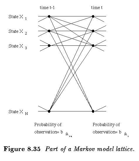
- We reconstruct the system evolution by imagining an N x T lattice of states; at
time t we occupy one of the N possible X_i in the t^th column.
- States in neighboring columns are connected by transition probabilities
from the A matrix, but our view of this lattice is attenuated by the
observation probabilities B.
- The task is to find the route from the first to the T-th column of maximal probability,
given the observation set.


- Here, equation (8.50) initializes the first lattice column, combining the
pi vector with the first observation.
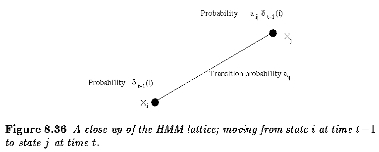
- Equation (8.51) is a recursion relation to define the subsequent column from the
predecessor, the transition probabilities and the observation; this gives
the i-th element of the t-th column, and informally is the probability of
the most likely way of being in that position, given events at time t-1.
- Equation (8.52) is a back pointer, indicating where one is most likely to
have come from at time t-1 if currently in state i at time t (see next
Figure).
- Equation (8.53) indicates what the most likely state is at time T, given
the preceding T-1 states and the observations.
- Equation (8.54) traces the back pointers through the lattice, initializing from
the most likely final state.

- A simple example will illustrate this; considering the weather transition probabilities
(equation 8.47) and the seaweed observation probabilities (equation 8.48), we might
conjecture, without prior information, that the weather states on any given
start day have equal probabilities
- so pi = (1/3, 1/3, 1/3)
- Suppose now we imagine a weather observer in a closed locked room with a piece
of seaweed -- if on four consecutive days the seaweed is dry, dryish, soggy,
soggy
- The observer wishes to calculate the most likely sequence of weather states that
have caused these observations.
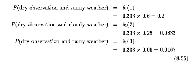
- Starting with the observation dry, the first column of probabilities becomes
(equation 8.50);

- The sunny state is most probable.
- Now reasoning about the second day, delta_2(1) gives the probability of observing
dryish seaweed on a sunny day, given the preceding day's information.
- For each of the 3 possible preceding states, we calculate the explicit probability
and select the largest (equation 8.51).

- Thus the most probable way of reaching the sunny state on day 2 is from
day 1 being sunny too;
- Accordingly, we record delta_2( 1 ) = 0.02 and store the back pointer phi_2
( 1 ) = 1 (equation (8.52).
- In a similar way, we find delta_2( 2 ) = .0188, phi_2 (2) = 1 and delta_2
( 3 ) = .00521, phi_2 (3) = 2.
- delta probabilities and back pointers may be computed similarly for the third
and fourth days; we discover delta_4(1) = 0.00007, delta_4(2) = 0.00055, delta_4(3)
= 0.0011
- -- thus the most probable final state given all preceding information, is
rainy.
- We select this (equation 8.53), and follow the phi back pointers of most
probable predecessors to determine the optimal sequence (equation 8.54).
- In this case, it is sunny, sunny, rainy, rainy, which accords well with
expectation given the model.
- HMM Learning
- The task of learning the best model to fit a given observation sequence is the
hardest of the three associated with HMM's, but an estimate (often sub-optimal) can
be made.
- An initial model is guessed, and this is refined to given a higher probability of
providing the observations in hand via the Forward-Backward algorithm or Baum-Welch
algorithm.
- This is essentially a gradient descent of an error measure of the current best
model, and is a special case of the EM (Estimate-Maximize) algorithm.
- Applications
- Early uses of the HMM approach were predominantly in speech recognition, where it
is not hard to see how a different model may be used to represent each word, how
features may be extracted and how the global view of the Viterbi algorithm
would be necessary correctly to recognize phoneme sequences through noise and
garble.
- HMMs are actively used in commercial speech recognizers.
- Wider applications in natural language processing have also been seen.
- The same ideas translate naturally into the related language recognition domain
of OCR and handwriting recognition.
- One use has been to let the underlying state sequence be grammatical tags, while
the observations are features derived from segmented words in printed and
handwritten text.
- The patterns of English grammar (which are not, of course, a first-order
Markov model) closely restrict which words may follow which others, and this
reduction of the size of candidate sets can be seen to assist enormously in
recognition.
- Similarly, HMMs lend themselves to analysis of letter sequences in text.
- Here, the transition probabilities are empirically derived from letter frequencies and
patterns (so for example, q is nearly always followed by u, and very rarely
by j), and the observation probabilities are the output of an OCR system.
- This system is seen to improve in performance when a second order Markov model is
deployed.
- At a lower level, HMMs can be used to recognize individual characters.
- This may be done by skeletonizing characters and considering the sequence of
stroke primitives to be a Markov process.
- Alternatively, vertical and horizontal projections of binarized character images may be
considered.
- Observed through noise, a Fourier transform of the projections is derived
as a feature vector, and a HMM for each possible character is trained using
the Baum-Welch algorithm.
- Unknown characters are then identified by determining the best scoring
model for features derived from an unseen image.
Last Modified: April 15, 1997
![[Go Back]](../IMAGES/next.gif)
![]()


![]()


![]()
![]()

