55:148 Digital Image Processing
55:247 Image Analysis and Understanding

Chapter 6, Part II
Shape representation and description: Contour-based shape representation and description

Chapter 6.2 Overview:

Chain codes
Simple geometric shape representation
Fourier transforms of borders
Boundary description using segment sequences
B-spline representation
Other contour-based shape description approaches
Shape invariants PE5.1

Contour-based shape representation and description

• Region borders must be expressed in some mathematical form.

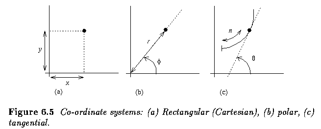
Chain codes

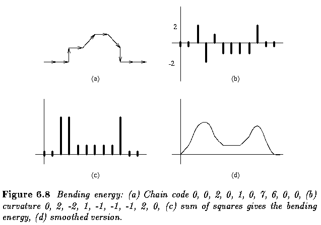
• Chain codes describe an object by a sequence of unit-size line segments with a given orientation.
• The first element of such a sequence must bear information about its position to permit the region to be reconstructed.

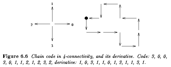
• If the chain code is used for matching it must be independent of the choice of the first border pixel in the sequence. One possibility for normalizing the chain code is to find the pixel in the border sequence which results in the minimum integer number if the description chain is interpreted as a base four number -- that pixel is then used as the starting pixel.
• A mod 4 or mod 8 difference is called a chain code derivative.

Simple geometric border representation

• The following descriptors are mostly based on geometric properties of described regions. Because of the discrete character of digital images, all of them are sensitive to image resolution.
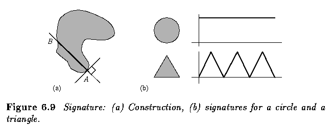
• Boundary length
• Curvature

• Bending energy

• Signature

• Chord

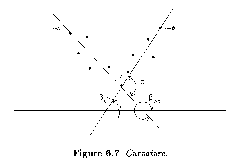
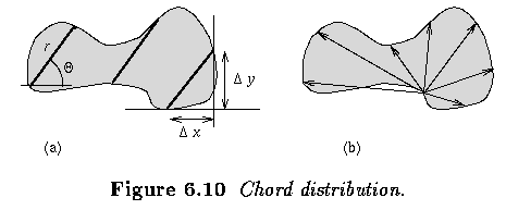
• Chord is a line joining any two points of the region boundary is a chord.
• Let b(x,y)=1 represent the contour points, and b(x,y)=0 represent all other points.

• Rotation-independent radial distribution:

• The angular distribution h_a(theta) is independent of scale, while rotation causes a proportional offset

Fourier transforms of boundaries

• Suppose C is a closed curve (boundary) in the complex plane.
• Traveling anti-clockwise along this curve keeping constant speed, a complex function z(t) is obtained, where t is a time variable.

• The coefficients T_n of the series are called the Fourier descriptors of the curve C. It is more useful to consider the curve distance s in comparison to time

• where L is the curve length. The Fourier descriptors T_n are given by

• The descriptors are influenced by the curve shape and by the initial point of the curve. Working with digital image data, boundary co-ordinates are discrete and the function z(s) is not continuous. Assume that z(k) is a discrete version of z(s), where 4-connectivity is used to get a constant sampling interval; the descriptors T_n can be computed from the discrete Fourier transform.

• The Fourier descriptors can be invariant to translation and rotation if the co-ordinate system is appropriately chosen.

• The coefficients a_n, b_n are not invariant, but after the transform

• r_n are translation and rotation invariant.
• To achieve a magnification invariance the descriptors w_n are used:

• The first 10 -- 15 descriptors w_n are found to be sufficient for character description.

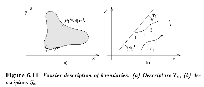
• A closed boundary can be represented as a function of angle tangents versus the distance between the boundary points from which the angles were determined

• The descriptor set is then

• The high quality boundary shape representation obtained using only a few lower order coefficients is a favorable property common to Fourier descriptors.

Boundary description using segment sequences

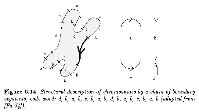
• If the segment type is known for all segments, the boundary can be described as a chain of segment types, a code-word consisting of representatives of a type alphabet.

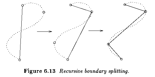
• A polygonal representation approximates a region by a polygon, the region being represented using its vertices. Polygonal representations are obtained as a result of a simple boundary segmentation.

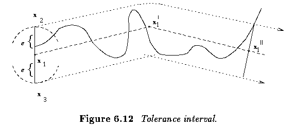
• Another method for determining the boundary vertices is a tolerance interval approach based on setting a maximum allowed difference e.

• Recursive boundary splitting.

• Boundary segmentation into segments of constant curvature or curve segmentation into circular arcs and straight lines is used.
• Segments are considered as primitives for syntactic shape recognition procedures.

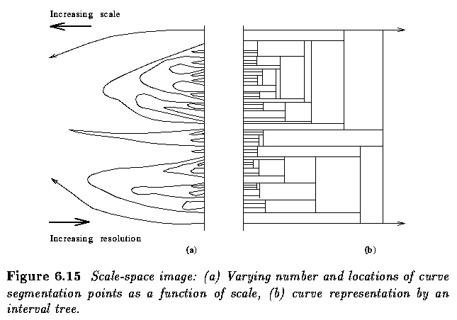
• Sensitivity of shape descriptors to scale is also important if a curve is to be divided into segments -- a scale-space approach to curve segmentation.
• Only new segmentation points can appear at higher resolutions, and no existing segmentation points can disappear.

• Fine details of the curve disappear in pairs with increasing size of the Gaussian smoothing kernel, and two segmentation points always merge to form a closed contour showing that any segmentation point existing in coarse resolution must also exist in finer resolution.
• Moreover, the position of a segmentation point is most accurate in finest resolution and this position can be traced from coarse to fine resolution using the scale-space image.

• A multiscale curve description can be represented by an interval tree.

B-spline representation

• Representation of curves using piecewise polynomial interpolation to obtain smooth curves is widely used in computer graphics.
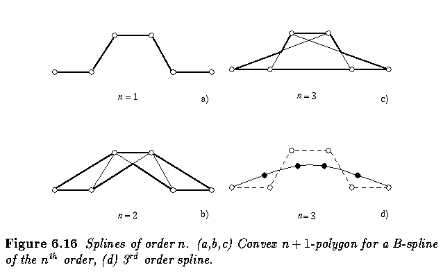
• B-splines are piecewise polynomial curves whose shape is closely related to their control polygon - a chain of vertices giving a polygonal representation of a curve.
• B-splines of the third-order are most common because this is the lowest order which includes the change of curvature.

• Splines have very good representation properties and are easy to compute:
• Firstly, they change their shape less then their control polygon, and do not oscillate between sampling points as many other representations do. A spline curve is always positioned inside a convex n+1-polygon for a B-spline of the n-th order.
• Secondly, the interpolation is local in character. If a control polygon vertex changes its position, a resulting change of the spline curve will occur only in a small neighborhood of that vertex.
• Thirdly, methods of matching region boundaries represented by splines to image data are based on a direct search of original image data.

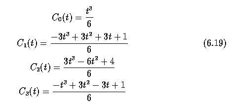
• Each part of a cubic B-spline curve is a third-order polynomial, meaning that it and its first and second derivatives are continuous. B-splines are given by

Other contour-based shape description approaches

• Many other methods and approaches can be used to describe two-dimensional curves and contours.

• The Hough transform has excellent shape description abilities.

• Region-based shape description using statistical moments is covered below.

• Fractal approach to shape is gaining attention in image shape description.

• Mathematical morphology can be used for shape description, typically in connection with region skeleton construction.

• Neural networks can be used to recognize shapes in raw boundary representations directly. Contour sequences of noiseless reference shapes are used for training, and noisy data are used in later training stages to increase robustness; effective representations of closed planar shapes result.

Shape invariants

• Shape invariants represent a very active current research area in machine vision.
• Importance of shape invariance has been known for a long time however it is somewhat novel approach in machine vision.
• Invariant theory is not new and many of its principles were introduced in the nineteenth century.

• Shape descriptors discussed so far depend on viewpoint, meaning that object recognition may often be impossible as a result of changed object or observer position.

• The role of shape description invariance is obvious -- shape invariants represent properties of such geometric configurations which remain unchanged under an appropriate class of transforms.

• Machine vision is especially concerned with the class of projective transforms.

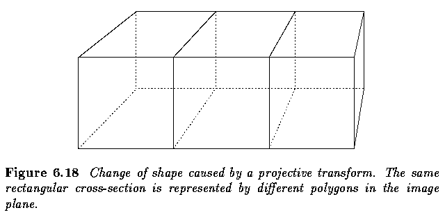
• Collinearity is the simplest example of a projectively invariant image feature. Any straight line is projected as a straight line under any projective transform.

• Similarly, the basic idea of the projection-invariant shape description is to find such shape features that are unaffected by the transform between the object and the image plane.

• A standard technique of projection-invariant description is to hypothesize the pose (position and orientation) of an object and transform this object into a specific co-ordinate system; then shape characteristics measured in this co-ordinate system yield an invariant description.
• However, the pose must be hypothesized for each object and each image which makes this approach difficult and unreliable.

• Application of invariant theory, where invariant descriptors can be computed directly from image data without the need for a particular co-ordinate system, represents another approach.

• Let corresponding entities in two different co-ordinate systems be distinguished by large and small letters. An invariant of a linear transformation may be defined as:
• An invariant, I(P), of a geometric structure described by a parameter vector P, subject to a linear transformation T of the co-ordinates x=TX, is transformed according to I(p)=I(P)|T|^w.
• Here I(p) is the function of the parameters after the linear transformation, and |T| is the determinant of the matrix T.
• In this definition, w is referred to as the weight of the invariant. If w=0, the invariants are called scalar invariants, which are considered below.

• Invariant descriptors are unaffected by object pose, by perspective projection, and by the intrinsic parameters of the camera.
• Several examples of invariants are now given.

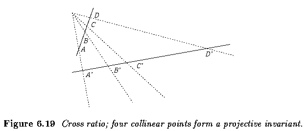
• Cross ratio:
• The cross ratio represents a classic invariant of a projective line.
• A straight line is always projected as a straight line. Any four collinear points A,B,C,D may be described by the cross-ratio invariant

• where (A-C) represents the distance between points A and C. Note that the cross ratio depends on the order in which the four collinear points are labeled.

Practical Experiment 5.1

1. Open the image shape-invariants.pgm or shape-invariants.tif using cantata (located in ~dip/examples/images.dir)
2. Determine coordinates of 4 collinear points from object type 1 and type 2 (corresponding within object types).
3. Calculate the invariant I (eq. 6.25) for the two shape classes - you may use the simple Matlab shape.m program (located in ~dip/examples/khoros.dir).
4. Are the invariants equal for smae objects imaged in different pose?
5. Are the invariants different for the two shapes?

Hint: For the star-like object, no collinar points exist directly. However, 4 coplanar lines can always be used to generate 4 collinear points.

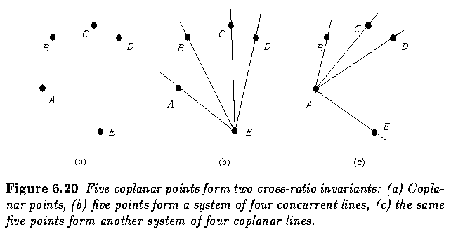
• A system of five general coplanar lines forms two invariants

where M_ijk=(l_i, l_j, l_k).

l_i=(l_i^1,l_i^2,l_i^3)^T is a representation of a line l_i^1x+l_i^2y+ l_i^3=0, where i is from interval [1,5], and |M| is the determinant of M.

If the three lines forming the matrix M_ijk are concurrent, the matrix becomes singular and the invariant is undefined.

• A system of five coplanar points is dual to a system of five lines and the same two invariants are formed.
• These two functional invariants can also be formed as two cross ratios of two coplanar concurrent line quadruples.
• Note that even though combinations other than those given in Figure may be formed, only the two presented functionally independent invariants exist.

• Plane conics:
• A plane conic may be represented by an equation

for x=(x,y,1)^T.

Then the conic may also be defined by a matrix C

• For any conic represented by a matrix C, and any two coplanar lines not tangent to the conic, one invariant may be defined

• The same invariant can be formed for a conic and two coplanar points.
• Two invariants can be determined for a pair of conics represented by their respective matrices C_1, C_2 normalized so that |C_i|=1

• For non-normalized conics, the invariants of associated quadratic forms are

• and two true invariants of the conics are

• Two plane conics uniquely determine four points of intersection, and any point that is not an intersection point may be chosen to form a five-point system together with the four intersection points.
• Therefore, two invariants exist for the pair of conics, as for the five-point system.

• Many man-made objects consist of a combination of straight lines and conics, and these invariants may be used for their description.
• However, if the object has a contour which cannot be represented by an algebraic curve, the situation is much more difficult.

• Differential invariants can be formed (e.g. curvature, torsion, Gaussian curvature) which are not affected by projective transforms.
• These invariants are local - that is, the invariants are found for each point on the curve, which may be quite general.
• Unfortunately, these invariants are extremely large and complex polynomials, requiring up to seventh derivatives of the curve, which makes them practically unusable due to image noise and acquisition errors, although noise-resistant local invariants are beginning to appear.
• However, if additional information is available, higher derivatives may be avoided.

• Stability of invariants is another crucial property which affects their applicability. The robustness of invariants to image noise and errors introduced by image sensors is of prime importance, although not much is known about this.
• Different invariants have different stability and distinguishing powers.

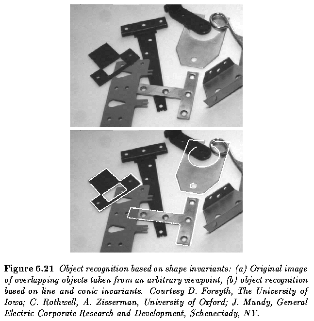
• An example of recognition of man-made objects using invariant description of four coplanar lines, a conic and two lines, and a pair of coplanar conics is given.
• The recognition system is based on a model library containing over thirty object models - significantly more than that reported for other recognition systems.
• Moreover, the construction of the model library is extremely easy; no special measurements are needed, the object is digitized in a standard way and the projectively invariant description is stored as a model.
• Further, there is no need for camera calibration. The recognition accuracy is 100% for occluded objects viewed from different viewpoints if the objects are not severely disrupted by shadows and specularities.

Last Modified: February 3, 1997