55:148 Digital Image Processing

Chapter 5, Part V
Segmentation: Advanced optimal border and surface detection approaches

Related Reading
Sections from Chapter 5 according to the WWW Syllabus.

Chapter 5.5 Overview:

Simultaneous detection of border pairs
Optimal surface detection

Advanced optimal border and surface detection approaches

• The concept of optimal border detection is extremely powerful and deserves more attention.
• In the following sections, two advanced graph-based border detection approaches are introduced.
• The first of them, the Simultaneous detection of border pairs, facilitates optimal identification of border pairs by finding a path in a three-dimensional graph.
• The second, the Optimal surface detection method, uses multi-dimensional graph search for highly efficient determination of surfaces in three- or higher-dimensional image data.

Simultaneous detection of border pairs

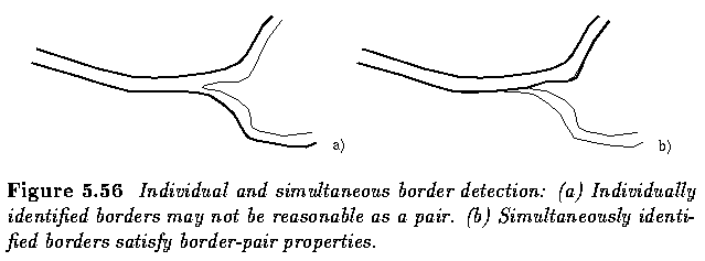
• If the goal is to determine borders of elongated objects, it may be advantageous to search for the pair of left and right borders simultaneously.
• Such an approach facilitates more robust performance if the borders forming the border pair are interrelated allowing information about one border to help identify the second.

• To search for an optimal border pair, the graph must be three-dimensional.

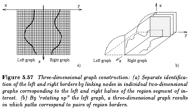
• Each parent node has nine successors corresponding to the possible combinations of change of positions of the left and right borders with respect to the centerline, thus forming a 3x3 successor window.

• With this successor rule, all paths through the 3D graph contain one and only one node from each profile plane in the 3D graph; that is, every path contains a single node derived from each of the left and right profile lines.

• The cost function for a node in the 3D graph is derived by combining the edge costs associated with the corresponding pixels on the left and right profiles in a way that allows the position of the left border to influence the position of the right border and vice versa.

• Similarly to the 2D case, the cost of a path in the 3D graph is defined as the sum of the costs of the nodes forming the path.

• The following cost function was found appropriate for description of border properties of a mutually inter-related border pair. Considering the cost minimization scheme, costs are assigned to nodes using the following function:

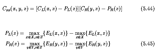
• Where Cs(x,y,z) is the sum of the costs for the left and right borders, Cpp(x,y,z) is a partial boundary cost, w(x,y) is a weighting function, and PL(z) and PR(z) are partial boundary costs.

• The edge costs of the left and right edge candidates located at positions x and y on profile z are inversely related to effective edge strength or other appropriate local border property descriptor E_L(x,z), E_R(y,z):

• X and Y are sets of integers ranging from 1 to the length of the left and right halves of the region profiles, and Z is the set of integers ranging from 1 to the length of the region centerline.

• To help avoid detection of regions adjacent to the region of interest, knowledge about the probable direction of the actual border may be incorporated into the local edge property descriptors E_L(x,z), E_R(y,z).

• Considering the individual terms of the cost function, the term C_s is the sum of the costs for the left and right border candidates and causes the detected borders to follow image positions with low cost values. It is given by:

• The C_pp term is useful in cases where one border has higher contrast (or other stronger border evidence) than the opposite border and causes the position of the low contrast border to be influenced by the position of the high contrast border. It is given by:

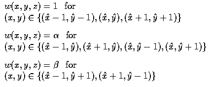
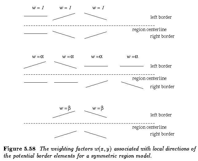
• The w(x,y,z) component of the cost function incorporates a model of the region boundary in a way that causes the positions of the left and right borders to follow certain preferred directions relative to the model.

• This component has the effect of discriminating against borders that are unlikely to correspond to the actual region borders when considered as a pair. This is accomplished by including a weighting factor that depends on the direction by which a node is reached from its predecessor.

• The influence of the region model is determined by the values of alpha and beta, typically alpha > beta.
• The larger the values of alpha and beta, the stronger is the model's influence on the detected borders.
• Typical values of alpha range from 1.2 to 1.8 and beta from 1.4 to 2.2.

• As the number of possible paths in a 3D graph is very large, the identification of the optimal path can be very computationally demanding.
• For example, for a 3D graph with xyz nodes, where z is the length in pixels of the region centerline, the number of possible paths is approximately 9^z.
• With conventional border detection, the number of possible paths in the two two-dimensional graphs of the same size is about 3^z.

• Improving the graph search performance is of great importance, and the P_L(z)+P_R(z) term in the cost function represents the lower bound heuristic, and does not influence the detected border; it does, however, substantially improve search efficiency if a heuristic graph searching approach is used.

• A second way to increase search efficiency - a multi-resolution approach.

• To enhance border detection accuracy, a multi-stage border identification process may also be included. The goal of the first stage is to identify reliably the approximate borders of the region segment of interest while avoiding detection of other structures. Having identified the approximate border positions, the second stage is designed to localize the actual region borders accurately.
• In the first stage, a relatively strong region model is used. Region boundaries identified in the low-resolution image are used in the second stage to guide the search for the optimal borders in the full-resolution cost image, as described in the previous paragraph. A somewhat weaker region model may be used in the second stage to allow more influence from the image data

Optimal surface detection

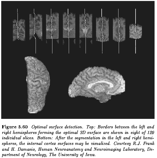
• If three-dimensional volumetric data are available, the task may be to identify three-dimensional surfaces representing object boundaries in the three-dimensional space.
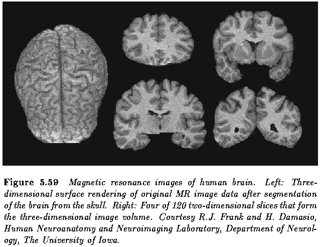
• Example: brain cortex visualization from three-dimensional magnetic resonance (MR) data sets of a human brain

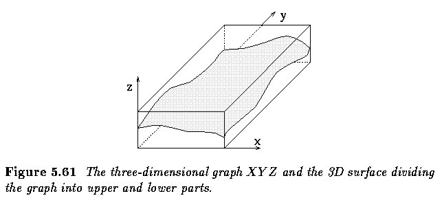
• Consider a 3D graph that corresponds in size with the 3D image data volume; the graph nodes correspond to image voxels.

• The legality of the surface is defined by the 3D surface connectivity requirements that depend on the application at hand, and the total cost associated with a surface can be calculated as the sum of individual costs of all nodes forming the surface.

• It should be possible to determine the optimal surface by application of optimal graph searching principles similar to those presented earlier. Unfortunately, standard graph searching approaches cannot be directly extended from a search for a path to a search for a surface.

• The search for an optimal surface results in combinatorial explosion of the task's complexity, and the absence of an efficient searching algorithm has until recently represented a limiting factor on 3D surface detection.

• An approach to optimal surface detection based on cost minimization in a graph was developed by Thedens and Fleagle that used standard graph searching principles applied to a transformed graph. While the method guaranteed surface optimality, it was impractical due to its enormous computational requirements.

• Frank and Dove developed a new approach to direct surfaces detection that is based on dynamic programming and avoids the problem of combinatorial explosion by introducing local conditions that must be satisfied by all legal surfaces.
• The approach can be generalized to searching higher-dimensional spaces

• The cost S of a surface is defined as

• The connectivity constraint guarantees surface continuity in 3D. The parameter N represents the maximum allowed change in the z-co-ordinate of the surface along the unit distance in x and y directions. If N is small, the legal surface is stiff and the stiffness decreases with larger values of N.

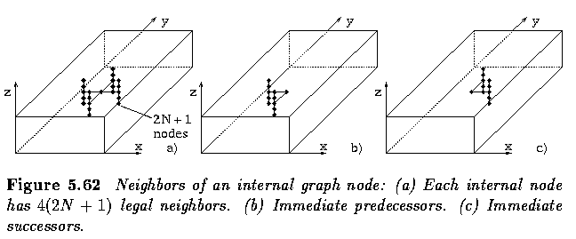
• Each internal node of the graph may have 4(2N+1) legal neighbors that have to be examined when constructing the 3D graph.

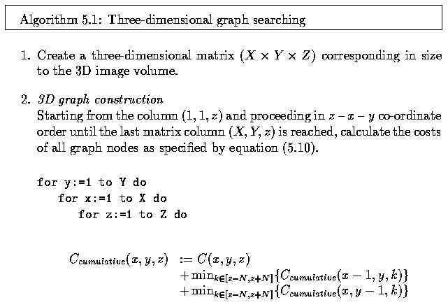
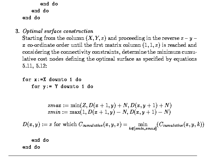
• The graph is searched starting from the vertical column with co-ordinates (1,1,z) in z -- x -- y co-ordinate order towards the column (X,Y,z).
• The cumulative surface cost is defined as the sum of the local cost associated with the node (x,y,z) and the sum of the two cost minima identified in the two columns constructed in the 3D graph that represent the immediate predecessors.

• The surface construction proceeds in the reversed z-y-x order.
• Propagation of the connectivity constraint guarantees the legality of the resulting surface. The z-coordinate of the surface-node in the (x,y) column, denoted by D(x,y) is defined as

• The backtracking process continues until the optimal node in the column (1,1,z) is identified.

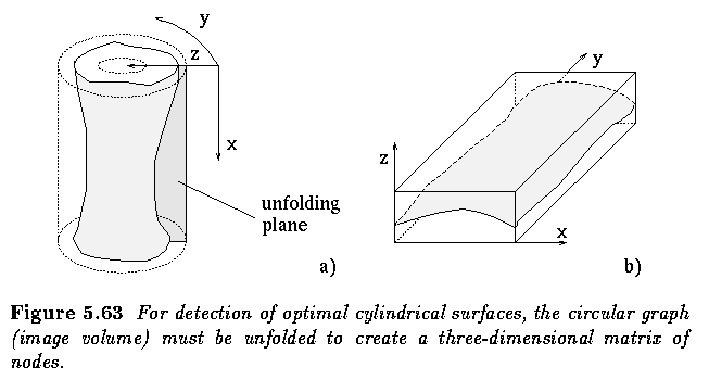
• Assuming a circular surface, the 3D graph can be constructed by unfolding the circular structure, considering the additional set of links from the set of graph columns (X,y,z) to the columns (1,y,z) to close the surface, and applying the graph-searching algorithm.
• However, the first and last row of optimal nodes may not satisfy the surface connectivity constraints. While it is possible to consider this constraint in the graph construction, a substantial increase in computational complexity results.
• There is a practical solution to the problem based on selecting a new cut-set of nodes along the y-co-ordinate to unfold the circular graph. Although not theoretically guaranteeing success under all circumstances, this approach has demonstrated practical applicability.

• In the brain segmentation example above, the cost function was based on inverted gray level values of the image voxels after the ventricles were three-dimensionally filled not to represent a large low-cost region.

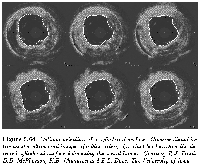
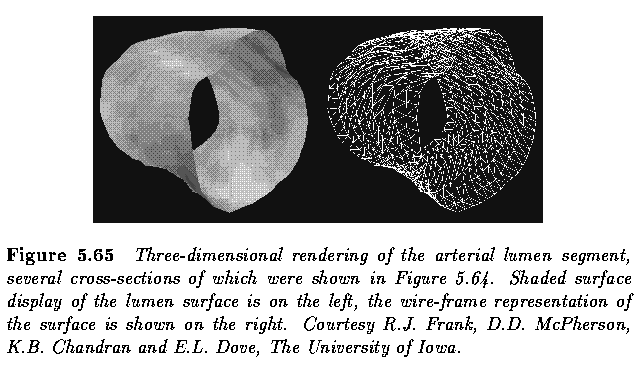
• In the IVUS data, the cost function was based on inverted edge strength and edge direction.

• The size of the graphs ranged from 100 x 25 x 10 for the intravascular ultrasound image sequences to 256 x 120 x 40 for the MR brain images.

Last Modified: January 27, 1997